Basics | A Quick Reference of the Evaluation Metrics in NLP

Overview

This set of evaluation metrics I discuss in this post is organized based on the typical tasks in NLP (see [1]); they are:

  • Sequence Classification
  • Token Classification (Tagging)
  • Generation: This category includes all tasks whose outputs are a sequence of tokens. For example, question answering, machine translation, text summarization and text simplification, and paraphrasing.
  • Retrieval
  • Regression

There is also a section dedicated to basic statistics, such as correlations, confidence intervals, and p-values.

Basic Statistics

Correlation

  • Choice of Correlation Measures

    We should choose Spearman correlation unless Pearson correlation is absolutely necessary (answer):

    • Pearson correlation is a parametric test for symmetric linear association; it has more stringent requirements.
    • Spearman correlation is a non-parametric test for monotinicity. It has lower requirement for data: data not normally distributed, data with outliers, ordinal or categorical data.
  • Number of Observation
    • The number of observations influence the confidence interval; smaller number of observations will make confidence interval wide. However, the small number of observations itself is not a problem; one real-life example is determining a new drug is effective on a small group of human subjects, where there may be only 5 or 6 people involved in the study.
    • Bootstrapping will not “turn a sow’s ear into a silk purse”: it only reduces confidence intervals (or significance level); it does not change correlation values (answer).

Sequence Classification

Confusion Matrix

The \mathbf{C}_{ij} means the number of samples of class i receive the prediction j; the rows are the true classes while the columns are the predictions.

  • When there are only two classes, we could define \mathrm{TN} = \mathbf{C} _ {11}, \mathrm{FP}=\mathbf{C} _ {12}, \mathrm{FN}=\mathbf{C} _ {21}, and \mathrm{TP}=\mathbf{C} _ {22}:

    Bases on these 4 numbers, we could define

    • $\mathrm{TPR}$, $\mathrm{FPR}$, $\mathrm{FNR}$, and $\mathrm{TNR}$: they are the normalized version of the confusion matrix on the true number of samples in each class.
    • Precision P and Recall R: we could compute these two numbers for each class; they are important in diagnosing a classifier’s performance.
Notation Formula
$\mathrm{TNR}$ $\frac{\mathrm{TN}}{\mathrm{N}}$
$\mathrm{FNR}$ $\frac{\mathrm{FN}}{\mathrm{N}}$
$\mathrm{FPR}$ $\frac{\mathrm{FP}}{\mathrm{P}}$
$\mathrm{TPR}$ $\frac{\mathrm{TP}}{\mathrm{P}}$
$P$ $\frac{\mathrm{TP}}{\mathrm{TP}+\mathrm{FP}}$
$R$ $\frac{\mathrm{TP}}{\mathrm{TP}+\mathrm{FN}}$
import numpy as np
from sklearn.metrics import confusion_matrix

y_true = np.array([1, 0, 1, 0, 1])
y_pred = np.array([1, 0, 1, 1, 0])

# raw counts
tn, fp, fn, tp = confusion_matrix(
    y_true=y_true,
    y_pred=y_pred
).ravel()

print(tn, fp, fn, tp)
# expected output: (1, 1, 1, 2)
# actual output: array([1, 1, 1, 2])

# tnr, fpr, fnr, tpr
tnr, fpr, fnr, tpr = confusion_matrix(
    y_true=y_true,
    y_pred=y_pred,
    normalize="true",
).ravel()

print(tnr, fpr, fnr, tpr)
# expected output: (1/2, 1/2, 1/3, 2/3)
# actual output: 0.5 0.5 0.3333333333333333 0.6666666666666666

  • We could use the code below to visualize a confusion matrix. Following the example above, we have:
import pandas as pd

df = pd.DataFrame(
    confusion_matrix(y_true, y_pred),
    index=labels
    columns=labels,
)

sns.plot(df)

Matthews Correlation Coefficient (MCC)

The Matthews Correlation Coefficient (MCC) (also called \phi statistic) is a special case of Pearson’s correlation for two boolean distributions with value {-1, 1}.

The range of MCC is [-1, 1], where 1 – perfect predictions, 0 – random prediction, and -1 – inverse prediction. It is better than F1 score (and therefore accuracy) as it does not have similar majority-class bias by additionally considering TN (remember that P=\frac{TP}{TP+FP}, R=\frac{TP}{TP+FN}, and F1=\frac{2PR}{P+R}=\frac{2TP}{2TP+FP+FN} and TN is not considered in F1).

Concretely, consider the following examples

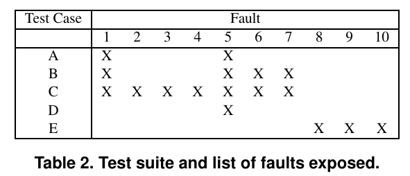
  • Example 1: Consider a dataset with 10 samples and y =(1, 1, \cdots, 1, 0) and \hat{y} = (1, 1, \cdots , 1, 1), then the F1=0.9474, MCC=0.
  • Example 2: Consider the use case A1 detailed in [3], given a dataset of 91 positive samples and 9 negative samples, suppose all 9 negative samples are misclassified and 1 positive sample is misclassified (i.e. TP=90, TN=0, FP=9, FN=1), then F1=0.95 while MCC=-0.03.

A potential issue when computing the MCC is that the metric is undefined when y is all 0 or all 1, and this will make either TP or TN undefined.
This issue also come with F1 score as it could be written as F1=\frac{2P\cdot R}{P+R}=\frac{2TP}{2TP+FP+FN} and it could not be computed when TP is undefined when all labels are 0.

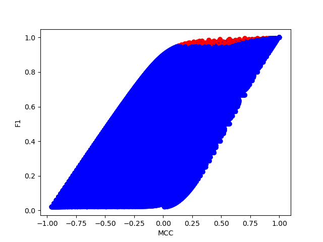
To have a better comparison between MCC and F1, consider a dataset with 100 samples, plot the F1 \sim MCC curve given different combinations of TP, FP, TN and FN using simulation. The dots colored red are those (1) achieve an more than 95% F1 score, and (2) correspond to a dataset where there are more than 95% positive samples. We could see that their MCC is relatively low.

Ranking

Typical ranking metrics include Mean Reciprocal Rank, Mean Average Precision, Precision, and Normalized Discounted Cumulative Gain (NDCG).NDCG is more comprehensive than other metrics as it considers the location of relevant items.

Metric Formula Note
MRR $\frac{1}{N} \sum _ {i=1}^N \frac{1}{r _ i}$ $r$ is the first relevant item for each query.
MAP@k $\frac{1}{N} \sum _ {i=1}^N \mathrm{AP}@k(i)$ $\mathrm{AP}@k(i) = \frac{1}{\text{# Relevant Items in Top-}k} \sum _ {i=1} ^ k \mathrm{P}@k(i) \cdot 1(i\ \text{is relevant})$.
P@k $\frac{1}{N} \sum _ {i=1}^N \mathrm{P}@k(i)$ $\mathrm{P}@k(i)$ is the ratio of relevant items in the total $k$ items for query $i$.
NDCG@k $\frac{\mathrm{DCG}@k}{\mathrm{IDCG}$k}$ $\mathrm{DCG}@k=\sum _ {i=1} ^ k \frac{\mathrm{rel} _ i}{\log _ 2 (i+1)}$, $\mathrm{IDCG}@k$ is the $\mathrm{DCG}@k$ for the ranking list of ideal order.

Suppose there are two queries q1 and q2, the returned documents have the following relevance list (1 as relevant and 0 as irrelevant):

q1 = [1, 0, 1, 0, 1]
q2 = [0, 0, 1, 1, 0]

Then we have the following results:

1 2 3 4 5 AP@5 DCG@5 IDCG@5
P@k for q_1 1 1/2 2/3 1/2 3/5 $\frac{1}{3}\times (1 + \frac{2}{3} + \frac{3}{5}) = 0.756$ $1 + \frac{1}{\log _ 2 4}+\frac{1}{\log_2 6}$ $1+\frac{1}{\log _ 2 3}+\frac{1}{\log _ 2 4}$
P@k for q_2 0 0 1/3 1/2 2/5 $\frac{1}{2}\times (\frac{1}{3} + \frac{1}{2})=0.417$ $\frac{1}{\log _ 2 4}+\frac{1}{\log_2 5}$ $1+\frac{1}{\log _ 2 3}$

Then, we have

  • P@5: \frac{1}{2} \times (\frac{3}{5} + \frac{2}{5}) = 0.5.
  • MAP@5: \frac{1}{2} \times (0.756 + 0.417)=0.587

Reference

  1. [2107.13586] Pre-train, Prompt, and Predict: A Systematic Survey of Prompting Methods in Natural Language Processing: This survey gives clear categories of NLP tasks: GEN , CLS, and TAG.
  2. Confusion matrix – Wikipedia: A comprehensive overview of a list of related metrics.
  3. The advantages of the Matthews correlation coefficient (MCC) over F1 score and accuracy in binary classification evaluation | BMC Genomics | Full Text (Chicco and Jurman).
  4. Calculate Pearson Correlation Confidence Interval in Python | Zhiya Zuo: The author writes a function that outputs Pearson correlation, p-value, and confidence intervals.
  5. sample size – Pearson correlation minimum number of pairs – Cross Validated

Meta | Formatting Requirements of Automated WordPress Publishing

Overview

There are two ways of publishing blogs onto a personal WordPress site:

  • Manual Copy and Paste
  • Automatic Publishing based on the solution introduced in GitHub (written in Chinese).

The second approach is preferred because of its almost complete automation. However, we need to follow the guidelines below to make sure that the content is rendered correctly when Markdown is converted to HTML.

Note that the HTML rendering does not seem to fully comply with the official guideline. It it therefore less useful to use a markdown linting tool, such as markdownlint by David Anson.

Guidelines

There has to be a newline before and after a list of bullets. Here we start a lot of complicated structures.

  • Always use 4 spaces rather than a tab when creating a lower level bullet point.
    • This is the test level 2.
      • This is the test level 3.
        • This is the test level 4.
  • If the contents in a bullet point has multiple paragraphs. Then it has to be organized as follows.

    There has to be 4 spaces before the subordinate paragraphs. For example, this paragraph is the second paragraph.

    This is the third paragraph of the bullet.

    • This is the second level bullet.

      This is a paragraph subordinate to the second level bullet.

Here we come back to the normal paragraph. For the best presentation of images and formulas:

  • They should not be subordinate to any bullet point; there should be no space before an image or a formula.
  • It is better to have a newline before and after an image or a formula.

a^2 + b^2 = c^2

Here we come back to the normal paragraph again.

Here we have a special note on the formula:

  • The rendering is likely to go wrong when there are multiple formulas with subscripts since the _ is also used for emphasizing in Markdown syntax (see the reported issue on GitHub). One workaround is adding a space before and after the _, i.e., replacing _ with <space>_<space>.

The following is the code used to generate the content above:

## Overview

There are two ways of publishing blogs onto a personal WordPress site:

- Manual Copy and Paste
- Automatic Publishing based on the solution introduced in [GitHub](https://github.com/zhaoolee/WordPressXMLRPCTools) (written in Chinese).

The second approach is preferred because of its almost complete automation. However, we need to follow the guidelines below to make sure that the content is rendered correctly when Markdown is converted to HTML.

Note that the HTML rendering does not **seem** to fully comply with the official guideline. It it therefore less useful to use a markdown linting tool, such as `markdownlint` by David Anson.

## Guidelines

There **has to** be a newline before and after a list of bullets. Here we start a lot of complicated structures.

- Always use **4 spaces** rather than a `tab` when creating a lower level bullet point.
    - This is the test level 2.
        - This is the test level 3.
            - This is the test level 4.
- If the contents in a bullet point has multiple paragraphs. Then it has to be organized as follows.

    There has to be **4 spaces** before the subordinate paragraphs. For example, this paragraph is the second paragraph.

    This is the third paragraph of the bullet.

    - This is the second level bullet.

        This is a paragraph subordinate to the second level bullet.

Here we come back to the normal paragraph. For the best presentation of images and formulas:

- They should not be subordinate to any bullet point; there should be no space before an image or a formula.
- It is better to have a newline before and after an image or a formula.

![](https://raw.githubusercontent.com/guanqun-yang/remote-images/master/2023/08/upgit_20230827_1693175262.png)

a^2 + b^2 = c^2

Here we come back to the normal paragraph again.

Talk Notes | Building End-to-End Content Moderation Pipelines in the Real World

[Website] – [Paper] – [Blog]

Note:
– The presenter of this talk is the lead author of the paper A Holistic Approach to Undesired Content Detection in the Real World.

Change Logs:

  • 2023-08-29: First draft.

Overview

There are two main iterations to build an end-to-end content moderator.
– Annotation Iteration: OpenAI outsource the most of the annotation iteration to external data providers. They also have internal expert annotators to provide the labels of the quality control set.
– Main Iteration: This is the bulk of the OpenAI’s contribution.

Annotation Iteration

  • Labeling guidelines need to be clarified and updated multiple times with more and more edges surface. The specifications from OpenAI are finally turned into training materials of their label providers to educate their annotators.
  • There should be sessions that
    • Calibrating the annotators by clarifying the annotation guidelines.
    • Auditing data that are flagged harmful either by the annotators or the model. Removing annotations from the annotator that has low per-category F1 scores. This process could be accelerated using cross-auditing with multiple annotators.

Main Iteration

There following are the diagrams that outline the steps above:

  • Step 0: Creating an initial dataset. This initial dataset includes those from “bad” (and unlabeled) subset of CommonCrawl, expert selected academic dataset, and zero-shot synthetic data from GPT-3 based on hand-crafted templates.
  • Step k-1: \cdots
  • Step k: In the iteration k, training a model \mathcal{M}_k based on GPT-series model using the standard cross-entropy loss.

One of the things the OpenAI could not solve well is the calibration.

  • Step k+1: Using \mathcal{M}_k to run inference on the unlabeled production data; the probabilities are used to select the subset for annotation. Three methods are compared:
    • Purely Random Sampling
    • Random Sampling for Samples Above a Threshold
    • Uncertainty Sampling

Active learning substantially improves the ratio of harmful contents in the user traffic (10 – 22 times).

After the subset is annotated, it is added back to the training set. Further, there is also synthetic data that is added to address the counterfactual bias.

  • Step k+2: Running the following steps to further improve the training data.
    • Overfitted Phrase Detection.
    • Mislabeling Detection.
  • Step k+3: Internal red teaming.
  • Step k+4: \cdots
  • Step -3:
  • Evaluating on the static test set.
  • A/B testing.
  • Step -1: Product release.

Here is a more detailed diagram; it is same as the one provided in the paper.

Future Direction

  • Dataset
    • A more systematic approach to create synthetic dataset. The current approach OpenAI uses is described ad-hoc.
    • Robustness to prompt injection and ciphers.
  • Continuous GPT-Assisted Red Teaming
  • Active Leraning
    • The current active learning approach relies on the model \mathcal{M}_k at Step k+1, which the model \mathcal{M}_k may not be able to generalize.
    • The presenter also mentions anomaly detection; it is not prioritized in OpenAI due to time constraint.

Reference

Reading Notes | Test Case Prioritization: An Empirical Study

Notes

[Semantic Scholar]- [Code] – [Tweet] – [Video] – [Website] – [Slide]

Change Logs:

  • 2023-08-27: First draft. This paper appeared at ICSM ’99. This conference was renamed to ICSME in 2014.
  • Test Case Prioritization (TCP) tries to order the test cases to optimize some objective, such as maximizing failure rates given a test budget of K or minimizing costs to obtain a coverage of \alpha.

  • TCP typically happens for regression testing, where we reuse the test suites and these test suites have historical statistics, such as actual failure rates on tests, coverage of branches or statements, and an estimation of probability of inducing bugs based on mutation.

Reading Notes | A Simple Fix to Mahalanobis Distance for Improving Near-OOD Detection

[Semantic Scholar] – [Code] – [Tweet] – [Video] – [Website] – [Slide]

Change Logs:

  • 2023-08-28: First draft. This paper is a preprint even though it uses the ICML template.

Method

This paper tries to patch the frequently used Mahalanobis Distance (MD) OOD detection metric for image classification tasks. The issue with the MD metric is that it fails for near-OOD scenario [3]. For example, separating examples from CIFAR-10 and CIFAR-100. The authors also try to argue this using eigen analysis.

Suppose we have a classification dataset of K classes \mathcal{D} = \cup_{k=1}^K \mathcal{D}_k, then we fit K+1 MD on each \mathcal{D}_k\ (k=1, \cdots, K) and \mathcal{D}, then for a test sample \mathbf{x}, a higher score below shows that it is more likely to be an OOD sample:

\mathrm{RMD}_ k(\mathbf{x}) = \mathrm{MD}_ k(\mathbf{x}) – \mathrm{MD}_ 0(\mathbf{x}),\quad
\mathrm{OODScore}(\mathbf{x}) = \min_ k \mathrm{RMD}_ k(\mathbf{x})

Experiments

  • The OOD detection performance is (1) asymmetrical, and (2) RMD does not significantly outperform MSP (Table 1).

    image-20230828124958624

Reference

  1. A Simple Unified Framework for Detecting Out-of-Distribution Samples and Adversarial Attacks (NIPS ’18; 1.4K citations): This paper notes that the NNs tend to provide overly confident posterior distributions for OOD samples; this observation motivates the authors to propose the MD metric for OOD detection. The paper also draws the distinction between the adversarial samples and OOD samples.

  2. [1610.02136] A Baseline for Detecting Misclassified and Out-of-Distribution Examples in Neural Networks (ICLR ’17): This is the paper that tries to detect OOD samples using posterior distribution \arg\max_{k=1,\cdots, K} p(k\vert \mathbf{x}). The paper [1] improves upon it.

  3. [2007.05566] Contrastive Training for Improved Out-of-Distribution Detection: This paper strongly argues that the an OOD detection metric should work across the difficulty levels of detection tasks. Their proposed approach makes their metric more uniform. They propose the Confusion Log Probability (CLM) to measure the task difficulty. Specifically, they assume they have access to ID and OOD datasets \mathcal{D}_ \mathrm{in} and \mathcal{D}_ \mathrm{out} during training. Then,

  • Step 1: Training an ensemble of N_e classifiers on the union dataset \mathcal{D}_ \mathrm{in} \cup \mathcal{D}_ \mathrm{out}. Note that (1) the label space of these two datasets \mathcal{C}_ \text{in} and \mathcal{C}_ \text{out} are not necessarily same, (2) they need to hold out a test set \mathcal{D}_ \text{test} for Step 2, and (3) training a model ensemble is necessary for model calibration purposes (paper).

  • Step 2: Computing the CLM score as follows. A higher CLM score indicates that the domains of \mathcal{D}_ \text{in} and \mathcal{D}_ \text{out} are closer.

    $$
    \log\left( \frac{1}{\mathcal{D}_ {\vert\text{test}\vert}} \sum_{\mathbf{x} \in \mathcal{D}_ \text{test}} \sum_{k \in \mathcal{C}_ \text{in}} \frac{1}{N_e}\sum_{j=1}^{N_e} \mathcal{M}_ j(\mathbf{x}) \right)
    $$

Reading Notes | DeepGini – Prioritizing Massive Tests to Enhance the Robustness of Deep Neural Networks

[Semantic Scholar] – [Code] – [Tweet] – [Video] – [Website] – [Slide]

Change Logs:

  • 2023-08-27: First draft. This paper appears at ISSTA ’20.

Method

The core of solving a TCP problem is to come up with a metric that correlates to error rates on the the test set. The authors design the metric as follows:

\xi(t) = 1 – \mathbf{p}_ t^T\mathbf{p}_ t

where the \mathbf{p}_ t is the probability distribution of the test t. We could easily parallelize the computation of this metric using \xi(T) = \mathbf{1} – \mathrm{diag}(\mathbf{PP}^T), where \mathbf{P} is a matrix of (n_\text{sample}, n_\text{class}). For example, to reproduce the Table 2 in the paper, we have:

import numpy as np

P = np.array([
    [0.3, 0.5, 0.2],
    [0.1, 0.1, 0.8],
    [0.6, 0.3, 0.1],
    [0.4, 0.4, 0.2]
])

xis = 1 - np.diag(np.matmul(P, P.T))
# array([0.62, 0.34, 0.54, 0.64])

image-20230827182742854

Some comments on this metric:

  • This metric is equivalent to entropy as the only different is an additional log term and a scalar.
  • This metric is exactly the same as the Gini score used in the decision trees (see sklearn doc).

Evaluation Metrics

Average Percentage of Fault-Detection (APFD) was first defined in [2], which first proposes the test case prioritization problem. The example below comes from that paper.

Suppose we have a program of 10 known faults and a suite of 5 test cases; each test case is able to detect a subset of faults, then we have the following table:

A B C D E
Test Suites Used (x-axis) 1/5 2/5 3/5 4/5 1
Faults Detected (y-axis) 1/5 2/5 7/10 7/10 1

Then we could compute the APFD with the statistics provided (answer); this answer agrees with what is provided in the paper (Figure 1).

import numpy as np

xs = np.linspace(0, 1, 6)
ys = [0, 1/5, 2/5, 7/10, 7/10, 1]

apfd = np.sum(np.diff(xs) * (ys[:-1] + np.diff(ys)/2))
# 0.5

image-20230827163319793

For machine learning models, the APFD is defined differently as 1 – \frac{1}{kn} \sum_{i=1}^k o_i + \frac{1} {2n}, where k of the total n tests are misclassified, and o_i is the index of the first test that revealls i-th misclassified test.

Experiments

  • The experiments in the paper prioritize (1) the original test splits of some image classification datasets, and (2) the adversarial attacked versions of these datasets using standard approaches like FGSM.
  • There are two issues with the paper:
    • This paper does not consider the OOD test sets.
    • The paper tries to augment the training set with the attacked test examples to improve the classification accuracy. It is more sensible to augment the training sets with external annotated datasets.

Reference

  1. Regression testing minimization, selection and prioritization: a survey (published 2012; more than 1K citations).
  2. Test Case Prioritization: An Empirical Study (ICSM ’99; ICSM renamed as ICSME in 2014): This paper first proposes the test case prioritization problem and the APFD metric.

Reading Notes | Data Selection for Language Models via Importance Resampling

[Semantic Scholar] – [Code] – [Tweet] – [Video]

  • 2023-08-25: First draft. This paper is a preprint.

Problem Settings

The paper tries to solve the data selection problem for language model pretraining. Suppose a collection of high-quality samples x_ 1′ \cdots, x_ n’ have a distribution p, with another collection of N low-quality samples available; how could we sample a high-quality subset x_ 1, \cdots, x_ k\quad (k \ll N) with an underlying distribution q that approximates p?

Heuristic Classification

This is the approach used by GPT-3, EleutherAI’s Pile dataset, PaLM to select training corpus. Specifically,

  • Training a fasttext regression model f: \mathcal{X} \rightarrow [0, 1] using unigrams and bigrams from high-quality datasets.
  • Applying the trained classifier to the low-quality data collection and sampling x_ i if np.random.pareto(alpha) > 1 - score. alpha is chosen as 9 in the GPT-3 paper:

    We chose \alpha=9 in order to take mostly documents the classifier scored highly, but still include some documents that were out of distribution.

    Samples from the Pareto distributions are small; this makes most of the included samples high-quality.

Data Selection with Importance Resampling (DSIR)

The issue of the heuristic classification is that it does not explicitly model the underlying distribution q. Instead, the authors of DSIR explicitly model the distribution of a corpus as follows:

p(z; \gamma)=\prod_ {j=1}^{10000} \gamma_ j^{z_ j}

where

  • $z$ is a 10000-dimensional vector; its entries represent the index of the hashed unigrams and bigrams (with potential collisions).
  • $\gamma$ is the parameter to learn.

After learning the distributions p and q, we could assign a weight to each sample of the pool w_ i = \frac{p(z_ i)}{q(z_ i)},\ i =1, \cdots, N. We could then sample the pool with weights w_ 1, \cdots, w_ N until we have collected k samples. The authors sample the data without replacement and explain this choice theoretically. They could have explained it better, as deduplication is one key aspect for language model pretraining (Falcon paper).

Experiments

  • The average KL reduction strongly correlates (r = 0.89) with the accuracies on the downstream task (i.e., GLUE). The DSIR significantly improves the downstream accuracies. This correlation is a post-hoc justification of dataset modeling p(z;\gamma).

    The KL reduction is defined as following, where \hat{p} is target distribution, \hat{q} is the raw distribution, and p’ is the distribution of doing some data selection, including random selection, expert curation, and sampling with the proposed algorithm.

    \frac{1}{\vert \mathcal{T}\vert} \sum_{\hat{p} \sim \mathcal{T}} \mathrm{KL}(\hat{p} \parallel \hat{q}) – \mathrm{KL}(\hat{p} \parallel p’),\quad \mathrm{KL}(p\parallel q)= H(p, q) – H(p)

    There is \mathcal{T} because the authors are trying to evaluate the data selection methods; these methods could be applied to many different models. Therefore, there will be n scores for n data selection algorithms.

  • Continued pretraining on RoBERTa on domain-specific datasets sampled using the DSIR algorithm improves upon the model fine-tuned with datasets sampled with the baseline methods (Table 1, 2).

  • Training BERT from scratch using data sampled with the different sampling approaches and fine-tuning on GLUE shows the proposed selection algorithm’s advantages over the heuristic classification and random selection (Table 4).
  • It is important to make sure the domain of the pretraining dataset matches the deployment domain as (1) performance typically drops when the domain is different (Table 3), and (2) domain transfer is hard to predict (Figure 3).

Code

The implementation of the DSIR algorithm is straightforward:

  • Obtaining the Count Vector of a String

    A count vector of text could be obtained with get_ngram_info(text) (i.e., z = h(x)). The hash_buckets returns an integer of [0, 9999].

    from nltk import WordPunctTokenizer
    
    tokenizer = WordPunctTokenizer()
    def hash_buckets(string, num_buckets=10000):
      return int(abs(hash(string)) % num_buckets)
    
    def get_ngram_info(line, n=2, num_buckets=10000):
      words = tokenizer.tokenize(line.lower())
      # "i love it" be be converted to:
      # - unigrams: ['i', 'love', 'it']
      # - bigrams: [('i', 'love'), ('love', 'it')]
      unigrams, bigrams = words, list(zip(words, islice(words, 1, None)))
    
      counts = np.zeros(num_buckets, dtype=int)
      for unigram in unigrams:
          counts[hash_buckets(unigram, num_buckets=num_buckets)] += 1
      for bigram in bigrams:
          counts[hash_buckets(bigram, num_buckets=num_buckets)] += 1
      return counts
    
  • Obtaining the Importance Weight

    The code snippet reads each line from the Pile dataset and assigns a score logratio to this line. The logratio will be used for sampling.

    log_diff_dist = np.log(target_dist + 1e-8) - np.log(pile_dist + 1e-8)
    
    with open(path, 'r') as f:
      lines = f.readlines()
    
      for k, line in enumerate(tqdm(lines, miniters=1000000, maxinterval=1000000)):
          ex = json.loads(line)
          line = ex["contents"]
    
          curr_count = get_ngram_info(line, n=ngrams)
          logratio = np.inner(curr_count, log_diff_dist)
          logratios.append(logratio)
    
  • Sample Selection

    Gumbel distribution is used to model the distribution of maximum values. The authors use it here to make sure the sampling is done without replacement (i.e., Gumbel top-k trick).

    logratios = logratios
    logratios += np.random.gumbel(size=len(logratios))
    
    # select the samples with lowest logratios
    chosen_idxs = np.argpartition(-logratios, num_to_retrieve)[:num_to_retrieve]
    

Based on the functions above, we could write a simple unified function select_data_using_dsir(source_df, target_df, num_to_retrieve). This function is applicable to the scenario where both the source and target dataset are not too large and could be processed in memory.

def select_data_using_dsir(source_df, target_df, num_to_retrieve):
    source_texts = source_df.text.tolist()
    target_texts = target_df.text.tolist()

    source_count_vecs = [
        get_ngram_info(source_text) for source_text in tqdm(source_texts, desc="modeling source texts")
    ]

    source_dist = np.sum(source_count_vecs, axis=0)
    target_dist = np.sum(
        [get_ngram_info(target_text) for target_text in tqdm(target_texts, desc="modeling target texts")],
        axis=0
    )

    source_dist = source_dist / source_dist.sum()
    target_dist = target_dist / target_dist.sum()

    log_diff_dist = np.log(target_dist + 1e-8) - np.log(source_dist + 1e-8)
    logratios = np.array([
        np.inner(source_count_vec, log_diff_dist)
        for source_count_vec in tqdm(source_count_vecs, desc="retrieving source texts")
    ])
    logratios += np.random.gumbel(size=len(logratios))

    source_df["score"] = logratios
    chosen_idxs = np.argpartition(-logratios, num_to_retrieve)[:num_to_retrieve]

    return source_df.iloc[chosen_idxs]

source_dataset = load_dataset('yxchar/imdb-tlm', split="train")
target_dataset = load_dataset("yxchar/ag-tlm", split="train")

source_df = pd.DataFrame(source_dataset)
target_df = pd.DataFrame(target_dataset)

selected_source_df = select_data_using_dsir(source_df, target_df, num_to_retrieve=100)

Reading Notes | Out-of-Distribution Detection and Selective Generation for Conditional Language Models

Overview

The paper proposes to teach the encoder-decoder language models (the Transformers model on translation task and the PEGASUS model on summarization task) to abstain when receiving sentences substantial different from the training distribution; abstaining from generating some contents (more metaphorically, saying “I don’t know” when “I” really do not know) is indicates that the system is trustworthy; this practice improves the system safety.

Method

Given a domain-specific dataset \mathcal{D}_1 ={(x_1, y_1), \cdots, (x_N, y_N)} and a general-domain dataset (for example, C4) \mathcal{D}_0, the authors fit 4 Mahalanobis distance metrics using the representations of a model f(\cdot). The Mahalanobis distance is defined as \mathrm{MD}(\mathbf{x}; \mu, \Sigma) = (\mathbf{x} – \mu )^T \Sigma^{-1} (\mathbf{x} – \mu ); it is equivalent to -\log \mathcal{N}(\mu, \Sigma) up to a constant and a scalar difference.

Notation Fitting the Distance Metric On
$\mathrm{MD}_0(\cdot)$ $\mathcal{D}_0$
$\mathrm{MD}_\text{input}(\cdot)$ ${x_1, \cdots, x_N}$
$\mathrm{MD}_\text{output}(\cdot)$ ${y_1, \cdots, y_N}$
$\mathrm{MD}_\delta(\cdot)$ ${f(x_1), \cdots, f(x_N)}$

Then the authors use either of the following two metrics to compute the OOD score of a test sample z; the w is decoded output of z. The idea of using relative distance comes from authors’ previous work on selective classification (see [3]).

  • Input Relative MD (RMD) Score: \mathrm{RMD}_ \text{input}(z) = \mathrm{MD}_ \text{input}(z) – \mathrm{MD}_0(z).
  • Output Relative MD (RMD) Score: \mathrm{RMD}_ \text{ouput}(w) = \mathrm{MD}_ \text{output}(w) – \mathrm{MD}_\delta(w).

If the scores indicate that the test sample z is an anomaly, the language model abstains from generating actual w; rather, it generates preset content such as “I don’t know.”

Experiments

  • Perplexity should not be used for OOD detection alone because
    • The fitted PDFs of perplexities on different datasets (i.e., domains) mostly overlap (Figure 1).
    • When the averaged OOD scores increase, the Kentall’s \tau between perplexity and quality measure is (1) low and (2) decreases (Figure 4). If perplexity is a good measure, then the curve should be mostly flat.
    • It could be combined with the proposed metric (Section 4.3, 4.4).
  • The proposed metrics perform differently for different types of tasks: \mathrm{RMD}_ \text{input}(\cdot) is more suitable for translation task and \mathrm{RMD}_ \text{output}(\cdot) is more suitable for summarization task. This may be because the summarization task is more “open-ended” than translation task.

  • The distance between domains could be quantitatively measured with the Jaccard similarity of n-grams (1 through 4 in the paper) (Table A.10). This is used to quantify the task difficulties as the authors define “near OOD” and “far OOD” domains (Table 1).

References

  1. [1705.08500] Selective Classification for Deep Neural Networks

  2. [1612.01474] Simple and Scalable Predictive Uncertainty Estimation using Deep Ensembles: This paper works on predictive uncertainty of deep classification models. Their proposed approach tries to approximate the state-of-the-art Bayesian NNs while being easy to implement and parallelize.

  3. [2106.09022] A Simple Fix to Mahalanobis Distance for Improving Near-OOD Detection: For a classification problem of K classes, we could fit K class-dependent Gaussian and 1 background Gaussian. Then we could use these (K+1) Gaussians to detect anomalies: a negative score in class k indicates that the sample is in the domain k and a positive score means it is OOD; a more positive score shows that the sample deviates more from that domain.

Summary | Reinforcement Learning Basics

Overview

The goal of reinforcement learning is to learn a policy \pi(a\vert s) = \Pr\left[ A=a\vert S=s\right] so that the agent will know what to do at each state s to maximize the expected cumulative reward it could receive in the future N steps (these steps are called an “episode”):

Q_\pi(s_t, a_t)
= \mathbb{E}_\pi \left[ U_t \vert S_t=s_t, A_t=a_t\right]\
= \mathbb{E}_\pi \left[ \sum_{k=0}^{N-t} \gamma^k R_{t+k} \vert S_t=s_t, A_t=a_t\right]

Under the hood, there is an unknown state transition function p(s’\vert s, a) = \Pr\left[ S’=s’\vert S=s, A=a\right] that is governed by the environment. What we could observe is a list of triplets (s_1, a_1, r_1) \rightarrow (s_2, a_2, r_2) \rightarrow \cdots (aka. “trajectory”); we could use collect the trajectory data to train the agent to find the best polity for it to execute.

As value function V(s) = \sum_a \pi(a\vert s) Q_\pi(s, a), there are three ways to maximize V(s):

Goal Model Category
Value-based Learning optimal action-value function Q^*_\pi(s, a) DQN + TD Off-policy
Policy-based Learning optimal policy function \pi^*(a\vert s) REINFORCE (or policy-gradient algorithm) On-policy
Hybrid Learning both policy and value Actor-Critic

Here is the distinction of on-policy and off-policy algorithms (answer):

  • On-policy: The policy we are using to control the agent is the same as the policy we are trying to improve.
  • Off-policy: The policy we are using to control the agent is different as the policy we are trying to learn. For example, we could use a greedy policy or random policy to control the agent in the hope that we could learn a better policy than either random or greedy policy.

Value-Based

DQN + TD

The DQN tries to use a model (for example, a neural network) to approximate the an imaginary oracle Q^*(s_t, a_t) = \max_\pi Q_\pi(s_t, a_t) (aka. optimal action-value function); the optimal action-value function tells you which action is the best in an “averaged” sense.

The DQN could be trained with Temporal Difference (TD) algorithm. The idea of the TD algorithm is that the same objective could be computed with two ways:

  1. Pure estimation: q_t = Q(s_t, a_t; \mathbf{w}_t)
  2. A partial observation plus estimation (aka. TD target): y_t = r_t + \gamma \cdot \max_\pi Q(s_{t+1}, a; \mathbf{w}_{t}).

Then we try to update \mathbf{w}_t by minimizing the difference between q_t and y_t so that in future iterations the model will perform better:

\mathbf{w}_{t+1} = \mathbf{w}_ t – \alpha \cdot (q_ t – y_ t) \cdot \frac{\partial Q(s_ t, a_ t;\mathbf{w})}{\partial \mathbf{w}} \rvert_{\mathbf{w} = \mathbf{w}_t}

The following are the steps for DQN + TD algorithm:

  • Step 1: Observe state s_t and perform an action a_t.
  • Step 2: In this step, we obtain three things:
    • Two estimations for the same target: q_t = Q(s_t, a_t;\mathbf{w}_ t) and y_t=r_t + \gamma \cdot \max_a Q(s_{t+1}, a;\mathbf{w}_t)
    • The gradient of the value network: \mathbf{d}_ t = \frac{\partial Q(s_ t, a_ t; \mathbf{w})}{\partial \mathbf{w}}\rvert_{\mathbf{w} =\mathbf{w}_ t}.
  • Step 3: Update the policy network: \mathbf{w}_ {t+1} = \mathbf{w}_ t – \alpha \cdot (q_t – y_t)\cdot \mathbf{d}_ t. This update happens every time we observe a reward.

Policy-Based

Overview

  • If both the actions and states are discrete and there are limited number of them, we could try to estimate the entries of a matrix of shape \vert S\vert \times \vert A\vert.
  • If either the state space is continuous but the action space is still discrete, we need to learn a distribution (typically a neural network) \pi(a\vert s; \theta) over the set of actions given each state s.

Policy-Gradient Algorithm

The goal is to maximize V(s;\theta) = \mathbb{E}_ A \left[Q_\pi(s, A)\right] = \sum_a \pi(a\vert s;\theta) \cdot Q_\pi(s, a) based on \frac{\partial V(s;\theta)}{\partial \theta} by learning a policy network \pi(a\vert s; \theta). After some derivation, this gradient is equal to:

\frac{\partial V(s;\theta)}{\partial \theta}=\mathbb{E}_ A\left[Q_\pi(s,A) \cdot \frac{\partial \log \pi(A\vert s;\theta)}{\partial \theta}\right]

Here are the steps for the policy-gradient algorithm:

  • Step 1: Observe state s_t and randomly sample an action a_t based on \pi(a\vert s_t;\theta_t).
  • Step 2: Evaluate the first part and the second part of the policy gradient:
    • $q_t \approx Q_\pi(s_t, a_t)$.
    • $\mathbf{d}_ {\theta, t} = \frac{\partial \log \pi(a_t\vert s;\theta)}{\partial \theta}\rvert_{\theta=\theta_t}$
  • Step 3: Update the policy network: \theta_{t+1} = \theta_t + \beta \cdot q_t \cdot \mathbf{d}_{\theta, t}

REINFORCE

REINFORCE algorithm is one instance of policy-gradient algorithms. It requires collecting the entire trajectory before training the policy network \pi(a\vert s;\theta).

Glossary

Name Formula Usage
Action-Value Function $Q_\pi(s, a)$ Action selection given a policy: how good if an agent picks action a in state s.
State-Value Function $V_\pi(s) = \mathbb{E}_ A\left[ Q_\pi(s, A) \right] = \sum_a \pi(a\vert s_t) \cdot Q_\pi(s_t, a)$ State evaluation given a polity: how good is the current situation s for a policy \pi.
$\mathbb{E}_ S\left[ V_ \pi(S) \right] = \mathbb{E}_ {S, A}\left[ Q_\pi(S, A) \right]$ Evaluation of a policy \pi.