Talk Notes | LLM and RLHF

[Talk on LLM] – [Talk on RLHF] – [Slides of LLM Talk] – [Tweet Thread of the LLM Talk]

  • The presenter Hyungwon Chung is a research engineer at OpenAI; he was with Google. He was doing mechanical engineering during Ph.D. that is completely irrelevant (aka. pressure-retarded osmosis) from machine learning.
  • The “Pretraining” section mostly comes from the LLM talk. The other sections are from the RLHF talk.

Pretraining

  • Functional Viewpoint of the Transformer LM

    The transformer could be viewed as a computation module that receives and outputs the matrices of size (b, d, l). All powerful LLMs are based on transformers. The interaction between tokens have minimal assumptions: each token could interact with any other token; this is done using a mechanism called “dot-product attention.”

    image-20231116111614647

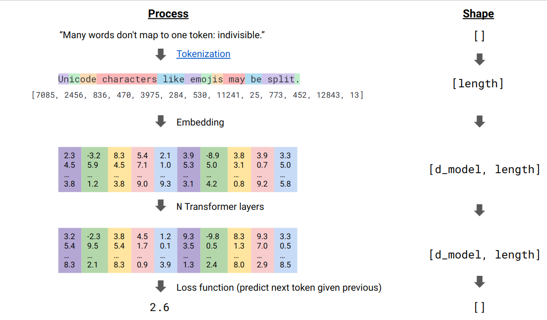
    For the sake of efficiency, the process above is done in batches. The only interdependence across the batch is finally the loss is divided by the batch size b.

    image-20231116111552954

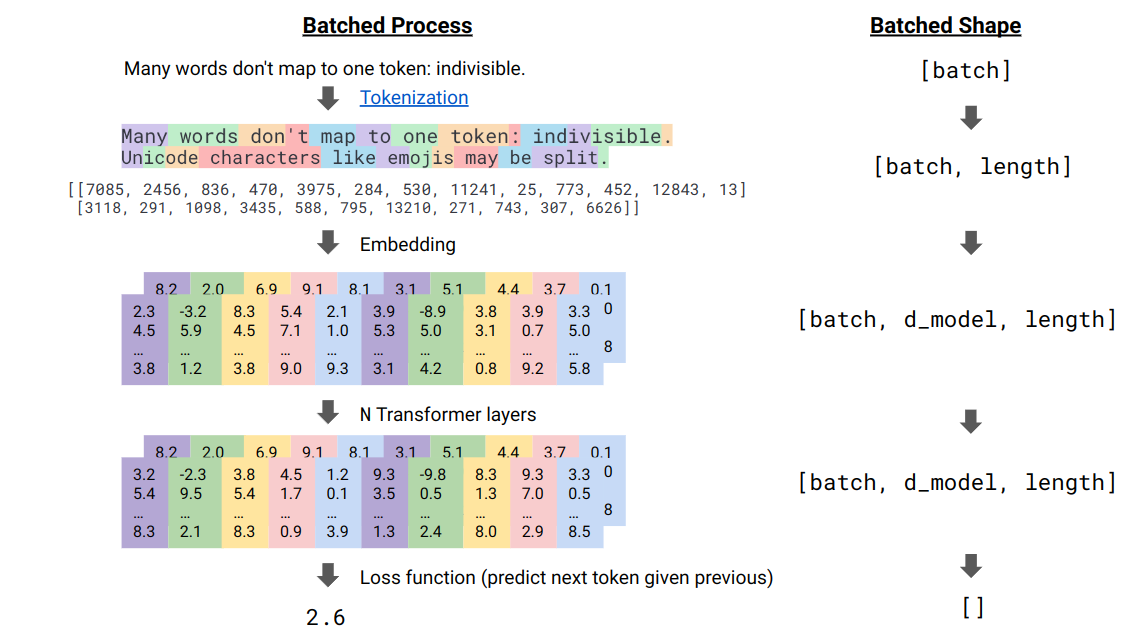
  • Scaling Transformers

    This means efficiently doing matrix multiplication with many machines (with matrices distributed on each and every machine) while minimizing the communication costs between machines.

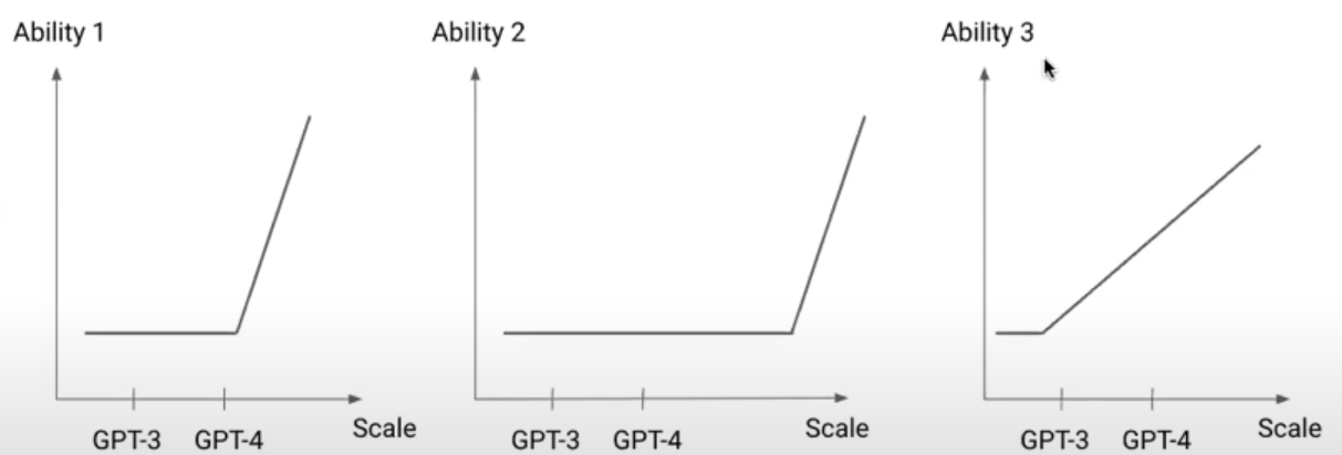
  • Scaling Law, Phase Change, and Emergent Abilities

    • An idea that does not work now may work when scaling up the model size. We need to constantly unlearn intuitions built on outdated or even invalidated ideas. We can update our intuition by reruning experiments that previously do not work on newer models and pinpointing what is new in these newer models.

Screenshot 2023-11-16 at 12.00.15 AM

  • Post Training
    • Users could not immediately communicate with the pretrained model as the training objective of pretraining is next token prediction. Prompt engineering mitigates this problem by setting up the ground for the LM to generate the relevant content.
    • Pretrained models always generate something that is a natural continuation of the prompts even if the content is malicious.

Supervised Fine-Tuning (SFT)

  • Instruction tuning is the technique that will almost universally beneficial to decoder only model and encoder-decoder model to improve their performances: the answer to “should I try instruction tuning” is almost always “yes.”

    Importantly, this is true even if we use encoder-only model as instruction-tuning provides a better initialization for “single-task” fine-tuning (see [2]). For example, we could use instruction-tuned BERT rather than regular BERT for various tasks.

    Pareto Improvements to Single Task Finetuning For both sets of Held-In and Held-Out tasks examined, finetuning Flan-T5 offers a pareto improvement over finetuning T5 directly. In some instances, usually where finetuning data is limited for a task, Flan-T5 without further finetuning outperforms T5 with task finetuning.

  • An Unified Architecture

    All tasks are unified with the single text-to-text format (proposed by T5). This was not obviously a valid choice because back to that time people do not believe LMs could “understand.”

  • Two Flavors of Instruction Tuning

    • Using Mixture of Academic Datasets: Flan and T0. The limitation of these models is that they could not generate longer texts due to the limitation of the academic datasets.
    • Using User Traffic: For example, InstructGPT and ChatGPT. The user traffics are unavaialble in the academic datasets (for example, “explain the moon landing to a six year old.”) as there is no way to evaluate them.
  • Task Diversity and Model Size are Important

    • The T0 by the presenter collects 1836 tasks; it is still the largest collections as of November 2023. The authors show the linear scaling law of model size and normalized performance on the held-out tasks. Further, when the number of tasks increase, the line is lifted upwards with a double digit gain. Further, it is important to have combine the non-CoT and CoT data together.
    • However, the performance quickly plateaus even when there are more tasks. This is likely due to limited diversity of academic datastes.
  • Inherent Limitation of Instruction Tuning

    For a given input, the target is the single correct answer (it could be called behavior cloning in RL); this requires formalizing correct behavior of a given input. However, this is hard or even impossible for inputs that look like the following:

    • Write a letter to a 5-year-old boy from Santa Clause explaining that Santa is not real. Convey gently so as not to break his heart.
    • Implement Logistic regression with gradient descent in Python.

    The issue is that (1) the correct answer may not be unique, and (2) it is hard or even impossible to provide the correct answer. However, the tension is that none of the existing functions could directly address these issues. The solution is using rewards in RL to address the problem.

RLHF

The lecture is based on the InstructGPT paper, which provides the foundational idea and popularize RLHF. There are many variants and extensions of this papers; they are easy to understand if we understand this foundational paper.

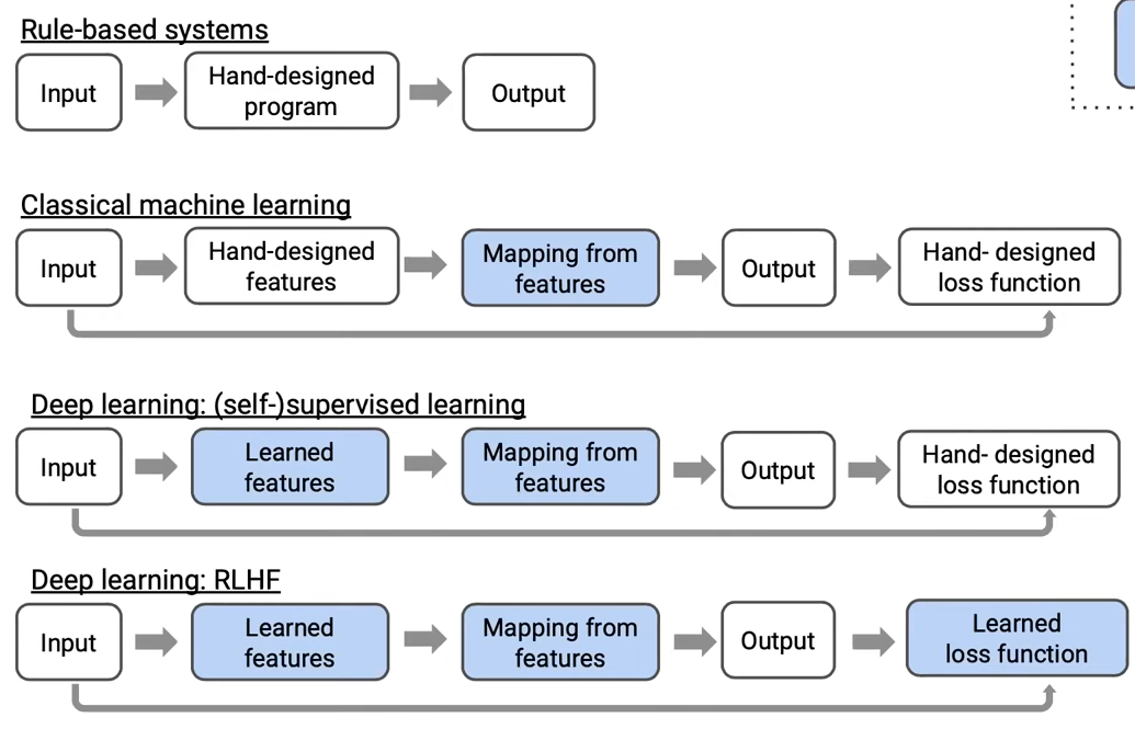
The goal of RLHF is encoding human preferences and (more generally) values. RLHF opens up a new paradigm of learning the objective function; the inductive bias from rule-based system to RLHF is gradually removed for more general use cases (the blue block refers to the learnable block within a system).

image-20231115234105819

Reward Model (RM)

The intuition of training a reward model is It is difficult to evaluate open-ended generation directly, but it is easier to compare two completions.

The reward model r(x, y;\phi) is the SFT model that replaces the last layer with a layer that outputs a scalar; it could also be done differently like taking the probability of [CLS] token, etc. As long as the model outputs a scalar, how exactly we model this process is less relevant.

Let p _ {ij} be the probability that the completion y _ i is better than y _ j (here the order matters), then based on the old Bradley-Terry model; the function r(\cdot) models the strength of the sample. Note that it is likely both y _ i and y _ j are bad, then the goal is to choose the one that is relatively better.
\log \frac{p _ {ij}}{ 1 – p _ {ij}} = r(x, y _ i ; \phi) – r(x, y _ j; \phi),\quad p _ {ij} = \sigma( r(x, y_i;\phi) – r(x, y _ j; \phi))

Then we want to find \phi so that the sum of the probabilities is maximized: \max _ \phi \sum _ {x, y _ i, y _ j \in D} \log p _ {ij}.

Note that there are some issues with the reward modeling; there are many ways to improve this scheme:

  • The scheme above does not model how much y _ i is better than y _ j.

Policy Model

Once we have the reward model r(\cdot), we could use that to update the parameters of the language model itself \pi _ \theta. Specifically, we would like to maximize the following. Note that the prompt X=(X _ 1, \cdots, X _ S) are from academic datasets or user traffic and completion Y = (Y _ 1, \cdots, Y _ T) are sampled from the language model \pi _ \theta; the reward model is fixed in this process.
J(\theta) = \mathbb{E} _ {(X, Y)\sim D _ {\pi _ \theta}} \left[ r(X, Y;\phi) \right]
The specific algorithm used to update \theta is PPO as it could give a stable gradient update. Here is the procedure:

  • Initialize the policy model to a SFT model.
  • Repeat the following:

    1. Sampling: Sampling prompts from the input datasets.
    2. Rollout: Generating the completion conditiong on the prompt with the current LM \pi _ \theta.
    3. Evaluation: Computing the reward of the input and the generated output using the (fixed) reward model r(x, y;\phi). Note that the reward model is not necessarily a model according to trl library, it could also come from a rule or a human.
    4. Optimization: Back-propagating the policy model and updating the parameter.

The explanation is alreay clear. To make the understanding more concrete, we could take a look at the MWE provided by trl library.

img

One issues (asked by He He) is that there might be distribution shift when applying the fixed reward model here; it could be an interesting problem to study: should we perodically update reward model (through something like continual learning) so that the distribution shift is mitigated?

Regularization

  • Preventing \pi _ \theta from Deviating Too Much from the SFT Model (Overfitting to RM or Reward Hacking)

    Adding the per-token penalty to prevent \pi _ \theta(Y\vert X) from growing too large compared to \phi _ \text{SFT}(Y\vert X). The intuition why this is important is that RM may model some human bias (for example, preference for longer texts) that may not be ideal for the task to solve.
    J(\theta) = \mathbb{E} _ {(X, Y)\sim D _ {\pi _ \theta}} \left[ r(X, Y;\phi) – \beta \log \frac{\pi _ \theta(Y\vert X)}{\pi _ \text{SFT}(Y\vert X)}\right]

Additional Notes

  • There is no reliable metrics to measure long generated texts; this is a problem not solved even for OpenAI.
  • The inputs are typically longer than outputs. This is one of the reasons why the models trained on the open-source datasets perform poor.
  • The easier tasks (for example, simple arithmetic like 3 + 2 =) is already solved pretty well by the pretrained models. The goal of the SFT and RLHF is to address the diverse and abstract prompts.
  • The RM is called preference model by Anthropic.
  • When we have k responses to the same input, we could form \binom{k}{2} sample pairs and put them in the same batch to avoid overfitting.
  • The Constitutional AI (CAI) by Anthropic almost automates everything during RLHF; the only human efforts involved is writing the constitution itself. For example, the model is tasked to generate prompts; these prompts are sent to train reward models.
  • np.einsum() is the extension of np.matmul().

Reference

  1. [2210.11416] Scaling Instruction-Finetuned Language Models (Chung et al., including Jason Wei)
  2. [2301.13688] The Flan Collection: Designing Data and Methods for Effective Instruction Tuning (Longpre et al.)
  3. [2009.01325] Learning to summarize from human feedback (Stiennon et al.): An example of reward hacking.
  4. [2212.08073] Constitutional AI: Harmlessness from AI Feedback (Bai et al.)

Talk Notes | Data-Centric AI

Overview

The following notes are the data-centric AI IAP course notes from MIT; Independent Activities Period (IAP) is a special four-week semester of MIT. The standard time for each lecture is 1 hour.

Lecture 1 – Data-Centric AI vs. Model-Centric AI

  • It is not hard to design fancy models and apply various tricks on the well curated data. However, these models and tricks do not work for real-world data if we do not explicitly consider the real-world complexities and take them into account. Therefore, it is important to focus on data rather than model.

    It turns out there are pervasive label errors on the most cited test sets of different modalities, including text, image, and audio. They could be explored in labelerrors.com.

  • To understand why data is important, we could think about kNN algorithm. The accuracy of kNN is purely based on the quality of datasets. However, the kNN is not a data-centric algorithm because it does not modify the labels.
  • Two Goals of Data-Centric AI

    Rather than modifying loss function, doing HPO, or changing the model itself, we do either of the following:

    • Designing an algorithm that tries to understand the data and using that information to improve the model. One such example is curriculum learning by Yoshua Bengio; in curriculum learning, the data is not changed but its order is shuffled.
    • Modifying the dataset itself to improve the models. For example, the confident learning (i.e., removing wrong labels before training the model) studied by Curtis Northcutt.
  • What are NOT Data-Centric AI and Data-Centric AI Counterpart

    • Hand-picking data points you think you will improve a model. \rightarrow Coreset Selection.
    • Doubling the size of dataset. \rightarrow Data Augmentation. For example, back-translation for texts, rotation and cropping for images. However, we need to first fix label errors before augmenting the data.
  • Typical Examples of Data-Centric AI

    Curtis Northcutt cites Andrew Ng and other sources on the importance of data in machine learning ([1] through [3]). Here are some examples of data-centric AI:

    • Outlier Detection and Removal. However, this process relies on a validation process on which threshold to choose.
    • Label Error Detection and Correction
    • Data Augmentation
    • Feature Engineering and Selection. For example, solving XOR problem by adding a new column.
    • Establishing Consensus Labels during Crowd-sourcing.
    • Active Learning. I want to improve 5% accuracy on the test set but I could afford as little new annotated data as possible.
    • Curriculum Learning.
  • Data-Centric AI Algorithms are Often Superior to Model-Centric Algorithms

    The model centric approaches (i.e., training less on what a model believes are the bad subset of data) is a much worse idea than the data-centric approach (i.e., confident learning).

image-20231106162934431

  • Root-Causing the Issues – Models or Data
    • The model should perform well on the slices of data. Slicing means not only sampling data to a smaller number but also reducing the number of classes from a large number to a very small number. For example, rather than classifying images to 1000 classes, we only focus on performance on two classes.
    • The model should perform similarly on similar datasets (for example, MNIST datasets and other digits dataset).

Lecture 2 – Label Errors

Notation

Notation Meaning Note
$\tilde{y}$ Noisy observed label
$y ^ *$ True underlying label
$\mathbf{X} _ {\tilde{y} =i, y ^ {*} = j}$ A set of examples whose true label is j but they are mislabeled as i.
$\mathbf{C} _ {\tilde{y} =i, y ^ {*} = j}$ The size of the dataset above.
$p(\tilde{y} =i, y ^ {*} = j)$ The joint probability of label i and label j; it could be estimated by normalizing \mathbf{C}; it is indeed dividing each entry by the sum of all entries in the matrix \mathbf{X}.
$p(\tilde{y} =i\vert y ^ {*} = j)$ The transition probability that the label j flips to label i; it could also be called flipping rate.

Categories of Label Errors

When comparing the consensus crowd-sourcing labels and the final label in the dataset, there are 4 types of label errors:

  • Correctable: The given label is wrong and it could be corrected with crowd-sourcing. This is the type of label the lecture focus on detecting.
  • Multi-label: The given label and the consensus label are both right. However, more than one label in \mathcal{Y} could be used to label the samples. For example, an image with co-existence of laptop and humans that is incorrectly labeled as “laptop.”
  • Neither: The given label and the consensus label are both wrong.
  • Non-agreement: There is no way to tell whether the given label or the consensus label is correct.

There are also two categories of the label errors the presenter does not focus on:

  • Uniform Random Flipping p(\hat{y} = i \vert y ^ * = j) = \epsilon, \forall i\neq j: This will show as a symmetric \mathbf{X} matrix. It is easy to solve and this type of errors are unlikely to happen in the real world.
  • Instance-Dependent Label Noise p(\hat{y} = i \vert y ^ * = j, \mathbf{x}): This will require a lot of assumptions on the data distribution. Importantly, this type of label errors seldom happen in the real world.

Uncertainty

There are two sources of uncertainty:

  • Aleatoric Uncertainty: Label noise. It is the difficulty of an sample. This difficulty could come from incorrect label y or the strange distribution of \mathbf{x}.
  • Epistemic Uncertainty: Model noise. It is the model’s inability to understand the example. For example, the model has never seen similar examples before or the model class is too simple.

Confident Learning

The focus of the lecture is the correctable errors; it is defined in previous sections; the matrix \mathbf{X} is non-symmetric. Furthermore, the lecture will focus on samples with one label and one annotation.

  • Motivation of Using Confident Learning

    • Ranking samples by loss does not work. We could not find a loss threshold and claim the samples above this threshold are label errors.
    • Deep learning does not solve the label noise problem (despite many papers and many claims) because these problems try to solve the datasets polluted by uniform noise.
  • Assumption: Class-Conditional Label Noise
    p(\hat{y} \vert y ^ {_}; \mathbf{x} ) = p(\hat{y} \vert y ^ {_})

    • Interpretation: Given the true label, there is a constant flipping rate for the samples under that true label to other labels.
    • Rationale: A pig image often confused with a boar image but not other items such as “missiles” and “keyboards.” This tendency has nothing to do with what exactly a pig look like in an image but the similarities of the classes.
    • Motivation: This assumption is made because the LHS couples the aleatoric uncertainy and epistemic uncertainty and this assumption decouples these two uncertainties.
  • Confident Learning

    • For each of the class j, we could define a model’s self-confidence. If the self-confidence score of class j is low, but some of the samples have very high confidence, then we could say that there is something wrong with that label.

    t _ j = \frac{1}{ \vert \mathbf{X} _ {\tilde{y} = j}\vert } \sum _ {x \in \mathbf{X} _ {\tilde{y} = j}} \hat{p} ( \tilde{y} = j; \mathbf{x}, \theta)

    • For samples labeled with i, if its predicted probability for class j larger then t _ j, then this sample is likely mislabeled and we could assign it to the set. We could obtain this matrix in a cross-validation style. For example, if we have 3 folds, we use 2/3 of the data to train the model \hat{p} and use the remaining 1/3 to compute this matrix.
      \hat{ \mathbf{X} } _ {\tilde{y} = i, y ^ {*} = j} = { \mathbf{x} \in \mathbf{X} _ {\tilde{y} = i}: \hat{p} (\tilde{y} = j; \mathbf{x}, \theta) \geq t_j}
    • Example

      Suppose we know the t _ j for “dog”, “fox”, and “cow” are 0.7, 0.7, and 0.9. We have following predictions and labels. We could obtain a matrix that looks like one below. The off-diagonal entries correspond to labeling errors.

      $y ^ {*} = \text{dog}$ $y ^ {*} = \text{fox}$ $y ^ {*} = \text{cow}$
      $\hat{y} = \text{dog}$ 1 1 0
      $\hat{y} = \text{fox}$ 1 3 0
      $\hat{y} = \text{cow}$ 0 0 1

      Note the following:

      • The last sample does not contain any animal and it is not counted. This shows that this scheme is robust to outliers.
      • It is possible t _ j is very small but this will happen when there are many classes. In this case, the predicted probability for each class will also small.

      image-20231106204002280

  • Applications

    • Confident Learning + Ranking by Loss

      If we see there are in total k off-diagonal samples, then we could pick the top-k samples based on loss values.

    • Confident Learning + Ranking by Normalized Margin

      We could also rank by normalized margin for a specific class i; normalized margin is defined as following
      p(\tilde{y} = i) – \max _ {j\neq i} p(\tilde{y} =j; \mathbf{x} \in \mathbf{X} _ i)

    • Self-Confidence

      When p(\tilde{y}=i) is close to 1, then as far as the model could think, the sample is not likely to be a label error.

Theory of Confident Learning

  • The model-centric approaches (i.e., model reweighting methods) will still propagate the errors back to the weights. However, the data-centric approaches (i.e., pruning methods) does not have this problem.
  • We could prove that even if the model is miscalibrated (i.e., overly confident in some classes), the confident learning method is still robust.

Implications on Testing

  • When focusing on the subset of data whose labels could be corrected, more capable models (for example, ResNet-50 vs. ResNet-18) perform worse as they fit the random noise in the training set.

Lecture 8 – Encoding Human Priors

Human priors could be encoded (i.e., finding a function to represent) into the ML pipeline in two ways. During training time, it could be done using data augmentation. During test time, this is done through prompt engineering with an LLM.

  • Data Augmentation
    • Images: Flip, Rotation, Mobius transformation, Mixup. Mixup could be thought of as the linear interpolation of two images.
    • Texts: Back-translation.

cleanlab Library

Anatomy

  • Understanding Cross-Validation in cleanlab

    The cross-validation in cleanlab means the probabilities have to be the test scores. Specifically, if we have 3 folds, then what we will keep are the test prediction probabilities of each 1/3 fold using the model trained on the remaining 2/3 folds.

    This logic could be found in estimate_confident_joint_and_cv_pred_proba() in cleanlab/count.py; it is the most important functions for cleanlab. It is used in find_label_issues function in CleanLearning class; this class also inherits from sklearn.base.BaseEstimator. The code could be found here.

  • keras is Necessary to Port cleanlab and transformer

    • cleanlab requires an API that similar to sklearn.
    • As of 2023-11-08, neither transformer or sklearn team provides a solution to port each other (except a less relevant library called skops that is about sharing sklearn models to HuggingFace hub; also see news). We therefore need to rely the keras-based code from cleanlab official tutorial that fine-tunes a TF-based bert-base-uncased to find label errors in imdb dataset.
    • The complete script is available here.

Example

In the official demo that tries to find label errors in the imdb dataset, the authors use a simple MLP as the base model. The following (confusing at the first look) code indeed tokenize the texts into fixed length vectors (i.e., sequence_length).

import re
import string

import tensorflow as tf
import tensorflow_datasets as tfds
from tensorflow.keras.layers import TextVectorization

raw_train_ds = tfds.load(name="imdb_reviews", split="train", batch_size=-1, as_supervised=True)
raw_test_ds = tfds.load(name="imdb_reviews", split="test", batch_size=-1, as_supervised=True)

raw_train_texts, train_labels = tfds.as_numpy(raw_train_ds)
raw_test_texts, test_labels = tfds.as_numpy(raw_test_ds)

max_features = 10000
sequence_length = 250

def preprocess_text(input_data):
    lowercase = tf.strings.lower(input_data)
    stripped_html = tf.strings.regex_replace(lowercase, "
", " ") return tf.strings.regex_replace(stripped_html, f"[{re.escape(string.punctuation)}]", "") vectorize_layer = TextVectorization( standardize=preprocess_text, max_tokens=max_features, output_mode="int", output_sequence_length=sequence_length, ) vectorize_layer.reset_state() vectorize_layer.adapt(raw_train_texts) # (N, sequence_length) train_texts = vectorize_layer(raw_train_texts).numpy() test_texts = vectorize_layer(raw_test_texts).numpy()

Additional Notes

  • “You are what you eat” is particularly relevant to the process of training machine learning models.
  • The data collection, labeling, and cleaning process could be called “data engine” or “data flywheel” in tech firms (blog).
  • The benefits of data-centric AI is that it disentangle the effects of data and modeling. Previously, we blindly trust the labels and efforts (including using larger models, changing loss functions, doing HPO) to improve the performance may only end up fitting the noise. If we make the data clean, we could identify what are the truly useful techniques and what are not.
  • cleanlab could not only flag the label issues but also automatically fix the top label issues. (blog).

    Here we use Cleanlab Studio’s Clean Top K feature, which allows us to automatically correct the top most severe issues detected in our dataset with an automatically suggested label (inferred to be more suitable for each example than its original label in the dataset).

Reference

  1. Why it’s time for ‘data-centric artificial intelligence’ | MIT Sloan
  2. Bad Data Costs the U.S. $3 Trillion Per Year (Harvard Business Review)
  3. Bad Data: The $3 Trillion-Per-Year Problem That’s Actually Solvable | Entrepreneur
  4. [1710.09412] mixup: Beyond Empirical Risk Minimization (Zhang et al., ICLR 2017)

Research Notes | Resource Central

Overview

The links I dump into Zotero or the bookmark manager software will be quickly forgotten if they are not revisited soon. This repository serves as a quick reminder that document all the links (1) I have collected, and (2) I have revisited and believed it should have been revisited eariler.

Basics

Research

Talk Notes | ACL 2023 Tutorial – Retrieval-based Language Models and Applications

[Zoom Recording] – [Website and Slides] – [Proposal] – [Q&A] – [Backup Recording]

  • This tutorial is given by Akari Asai, Sewon Min, Zexuan Zhong, and Danqi Chen

Overview

RALM is an LM that uses external databases in the test time.

The motivation of RALM is the pessimism about the current editing-based approaches. If we are able to edit the LLMs as fast as CRUD operations on databases, the retrieval-based approaches and editing-based approaches are comparable.

Moreover, these parametric LMs are fundamentally incapable of adapting over time, often hallucinate, and may leak private data from the training corpus. […] Retrieval-based LMs can outperform LMs without retrieval by a large margin with much fewer parameters, can update their knowledge by replacing their retrieval corpora, and provide citations for users to easily verify and evaluate the predictions.

Besides ease of updating knowledge, the retrieval-based approaches also have following advantages:

  • Traceability, Verifiability, Interpretability, and Controllability: They mean the same thing for RALMs.
  • Privacy and Copyright: The LMs are only responsible for making inference. The more relevant documents are stored in the databases.

There are some use cases where the RALMs are most suitable:

  • Long-tail: For example, “Where is the Toronto zoo located?”
  • Knowledge Update: For example, “what is the population of Toronto metropolitan area in 2000?”
  • Verifiability, Factuality, and Hallucination
  • Parameter-Efficiency: RALMs could improve performance of smaller LMs and make them competitive with larger ones.
  • Parameter Update: We do not have to update the model itself when we could update the database.
  • OOD Generalization

Architecture

Three elements of RALMs:

  • What to Retrieve? What is the minimal unit for retrieval. The choices could be token, document, or text chunk.
  • How to Use the Retrieval Results? Input, output, or somewhere in between?
  • When to Retrieve? Only once, every token, or somewhere in between?

image-20231102223928224

  • REALM is one of the first works in RALM. The goal is improving MLM LM pretraining. The followup papers include DPR, RAG, Atlas; they all focus on knowledge intensive tasks:

    • DPR
    • RAG
    • Atlas
  • Retrieval-in-context LM

    • REPLUG: The prompt is used to retrieved a set of documents; these documents are then prepended to the prompt and form an ensemble to predict the new tokens.
    • Ram et al.: We do not have to use the entire prompt as query. It may be better to use more recent tokens (due to higher relevance to the tokens to generate) as long as they are not too short.

      Further, we may want to retrieve more often. For example, after we have already generated some tokens, it is time to retrieve again for the next batch of new tokens.

  • RETRO

    • Used in the intermediate layer. Specifically, each prompt is chunked into multiple pieces and sent to retrieve some results; these results are sent into the LM through a specially design attention mechanism. The authors also consider some parallelization techniques for the sake of efficiency.
    • Another orthogonal finding of this paper is that the scale of the datastores are important.
  • kNN-LM

    • Using the test prefix to query for the prefixes that are already continued with new tokens. The token to generate will be an linear interpolation between the actual generated new tokens and the new tokens that belong to the best match prefix.
    • The motivation of this design is that the text representations of the entire sentences could be quite different even though the same word appears in it. For example, the word “torch” and “cheap.”

      Comment: The motivation of this design is dubious. Furthermore, the interaction between the input and the retrieved results is limited.

  • Extensions to kNN-LM

    • Adaptive Retrieval. Whether the retrieval is enabled depends on the confidence of the outputs. For example,
      • FLARE and He et al. More specifically, the \lambda in kNN-LM could be a function of confidence.
      • Alon et al.
  • Entities as Experts

    • Entities could be represented as dense vectors and incorporated into the intermediate layers of a model.
    • Extension: Mention Memory
Paper What When How Note
REALM Chunks Once Input Used in real-world applications such as you.com, Bing Chat, and perplexity.ai.
Retrieve-In-Context LM Chunks Every n Tokens Input Used in real-world applications such as you.com, Bing Chat, and perplexity.ai.
RETRO Chunks Every n Tokens Intermediate
kNN-LM Tokens Every Token Output
FLARE Chunks Adaptive Input
Adaptive kNN-LM (He et al., Alon et al.) Tokens Adaptive Output
Entities of Experts; Mention Memory Entities or Entity Mentions Every Entity Mention Intermediate
Wu et al., Bertsch et al., Rubin & Berant Chunks from Input Once or Every n Tokens Intermediate All methods above retrieve from external text. We can also retrieve from the book-length input.

Training

We could update (1) the LM itself and (2) retrieval model. However, training either of them is difficult as (1) LM is typically large and therefore expensive to make parameter updates (2) index has to be updated every time we update the the encoder and this is proportional to the number of documents in the database.

There are 4 strategies for training the RALMs. Independent and sequential training render no or weak dependence between the LM and RM but the system performance is not as strong as the joint training (i.e., training the LM and RM jointly); the downside of the joint training is the requirement for a special training protocl.

Independent Training

Training LM and retrieval model independently. Each component could be improved separately; the improvement in each component will translate to the final improvement.

  • LM
  • Retrieval Model: It could be BM25 or DPR. BM25 does not need explicit training and the training of DPR is pretty straightforward. Note that the loss used to promote the correct pairs from the in-batch negatives is a type of contrastive learning.

    Besides DPR, another model is the contriver model (Izacard et al.), which is able to train in an unsupervised fashion.

Here are some examples of using this scheme:

  • kNN-LM: The retrieval model is fixed and only the LM is trained.
  • Ram et al.

Sequential Training

Sequential training means training one component first and then training the second component; the training of the second component depends the first component. As there are two components, we could either start from training the LM or the retrieval model.

  • RM \rightarrow LM: For example, RETRO.
  • LM \rightarrow RM: For example, REPLUG. Besides the ensemble prediction scheme, the authors further propose a method to fine-tune the retrieval model (dubbed as “LSR” by the authors) based on the feedback of the LM.

Joint Training with Asynchronous Index Update

Asynchronous index update means that we allow the index to “stale:” we do not reindex every document every time we update the encoder; rather, we only reindex the documents every T steps.

Joint Training with In-Batch Approximation

Applications

Questions

  • Where should we use RALMs.
  • Where should we plug in the RM + database.
  • Should we update the LM or RM.
  • What database should be used? Wikipedia, training data, or code documtation.
  • WebGPT and GopherCIte uses the Google search results as data store.
Task Method Database
DocPrompt Code Generation Prompting (Input)
Fine-Tuning LM
Code Documentation
KNN-Prompt Classification Prompting (Output) Wikipedia + CC
REPLUG Knowledge-Intensive Prompting (Input) Wikipedia + CC
ATLAS Knowledge-Intensive Fine-Tuning LM and RM Wikipedia + CC
GopherCite QA Fine-Tuning + RL on LM Google Search Results

Additional Notes

  • The backup video is downloaded based on the instruction documented here. Basically, we just need to replace the <cookie content> and <request url> with the content we obtain after F5 \rightarrow F12 in the browser.
youtube-dl -o video.mp4 --referer "https://zoom.us/" --add-header "Cookie: COOKIE_CONTENT" 'REQUEST_URL'

Reference

  1. Building Scalable, Explainable, and Adaptive NLP Models with Retrieval | SAIL Blog
  2. Atlas: Few-shot Learning with Retrieval Augmented Language Models (Izacard et al., 2022)
  3. Teaching language models to support answers with verified quotes (Menick et al., 2022)
  4. REPLUG: Retrieval-Augmented Black-Box Language Models (Shi et al., 2023)
  5. kNN-Prompt: Nearest Neighbor Zero-Shot Inference (Shi et al., 2022)
  6. Attributed Question Answering: Evaluation and Modeling for Attributed Large Language Models (Bohnet et al., 2023)
  7. DocPrompting: Generating Code by Retrieving the Docs (Zhou et al., 2022)
  8. REALM: Retrieval-Augmented Language Model Pre-Training (Guu et al., 2020)
  9. In-Context Retrieval-Augmented Language Models (Ram et al., 2023)
  10. Improving language models by retrieving from trillions of tokens (Borgeaud et al., 2022)
  11. Generalization through Memorization: Nearest Neighbor Language Models (Khandelwal et al., 2020)

Reading Notes | AutoGen – Enabling Next-Gen LLM Applications via Multi-Agent Conversation

Overview

Qingyun Wu’s Talk

  • The interaction between the users and the AutoGen system is critical for the system to be useful; fully autonomous systems are not trustworthy. For example, if the system does not deliver the outcome the user want, we could not know which step goes wrong.
  • In order for the system to be useful, the base models are important. We cannot use a very weak LM as one of the AI agents.
  • There are currently (as of 2023-11-01) no safety measures to make sure the system do not generate undesirable content.

Research Notes | Transformer from Scratch

Overview

This post aims to implements the the transformer model and its variant from scratch. It is based on the following posts:

  1. The Annotated Transformer (Harvard NLP)
  2. The Illustrated Transformer – Jay Alammar – Visualizing machine learning one concept at a time.
  3. GitHub – karpathy/minGPT: A minimal PyTorch re-implementation of the OpenAI GPT (Generative Pretrained Transformer) training: Anderj Karpathy also creates a 2-hour video describing the process he creates the model.

    GitHub – karpathy/nanoGPT: The simplest, fastest repository for training/finetuning medium-sized GPTs.: This is the optimized version of minGPT that is able to reproduce some of the mid-sized models, including a 1.3B GPT-2. Pretraining a 124M GPT-2 took 4 days on 8 A100 GPUs (each 40 GB).

  4. GitHub – nlp-with-transformers/notebooks: Jupyter notebooks for the Natural Language Processing with Transformers book

Research Notes | Machine Learning

Overview

The following notes are organized by and taken from the books below:

  • Hands-On Machine Learning with Scikit-Learn, Keras, and TensorFlow, 2rd Edition; this book’s 3rd edition has been released in 2022.

Dimensionality Reduction

The notion of “curse of dimensionality” does not arise solely regarding computation: more features makes the computation slow. It is also backed up by some theoretical observations. Specifically, consider the unit square, cube, or hypercube of 2, 3, through 10000 dimensions, we consider (1) when we sample one point, the probability it is within 0.001 to the border is 1 – (1 – 0.001) ^ d, (2) when we sample two points, the average distance of these two points is roughly \sqrt{d/6} (see answer).

This indicate that the in high dimensional space (1) any point is likely to be close to the border because it is easy for a point to be an extremist in one dimension with an increase in the number of dimensions, (2) the points are sparse; this sparsity could only be remedied by exponentially more samples with respect to dimension d, which is infeasible in practice.

Reading Notes | Towards Understanding Chain-of-Thought Prompting – An Empirical Study of What Matters

[Semantic Scholar] – [Code] – [Tweet] – [Video] – [Website] – [Slide] – [Poster]

Change Logs:

  • 2023-10-20: First draft. The paper appears at ACL 2023 as the best paper honorable mention.

Method

  • The experiments of this paper was done on text-davinci-002 with greedy decoding with temperature 0. The datasets they work on is quite small due to manual efforts required.
  • The paper focus on QA and arithmetic reasoning tasks; the authors introduce two concepts:

    • Bridging Objects
    • Language Template
  • The authors define the intermediate F1 scores for bridging objects. It is likely that the authors only accept generations that satisfy the predefined template and compute these metrics.
  • Observations:

    • The correctness of reasoning during CoT is not important.
    • Query should be (1) relevant and (2) follow the order of reasoning steps.
  • Additional Observations:

    • CoT does not make LLMs better; it unlocks the ability already learned by LLMs during pre-training. For example, the conclusions drawn on text-davinci-002 does not apply to Flan-PaLM; this is because Flan-PaLM has been fine-tuned on the two tasks.

      Given limited resources and an ability to fine-tune the model, we should include more and more data to pre-training or instruction tuning to improve the model rather than focusing the specific prompt engineering tricks.

Experiment

Additional Notes

Reference

Research Notes | Query Generation

Problem Statement

The paper [2] notes the difficulty of optimizing the query for neural retrieval models.

However, neural systems lack the interpretability of bag-of-words models; it is not trivial to connect a query change to a change in the latent space that ultimately determines the retrieval results.

The query generation aims to find out “what should have been asked” for a given passage. More formally, if we have a list of documents D that are aligned with our goal (or true underlying query) q, is it possible to search for its approximated version \hat{q} that returns D as relevant documents with high probability?

Background

  • Rocchio Algorithm for Query Expansion

    Rocchio algorithm is used by search engines in the backend to improve the user’s initial search queries. For example, if the initial search query is “beaches in Hawaii,” if the backend finds that many users click webpages (this is one type of pseudo relevance feedback, PRF) that contain the word “sunset,” then the word “sunset” will be added to the initial search query, making the real search query “beaches in Hawaii sunset.”

    There could be more nuanced PRFs than binary click and not-click action. For example, how long the users stay on a webpage, whether the user eventually returns to the search result page.

Adolphs et al., EMNLP 2022

There are two contributions of this paper:

  • Query Inverter: An inverter that converts embeddings back to queries.
  • Query Generation: A way to refine the initial generic query (plus a gold document) so that the gold passage will become one of the top ranked documents given a refined query.

Query Inverter

The authors use the GTR model to generate embeddings from 3M queries from the PAQ dataset [5], thus forming a datasets {{(q_i, \mathbf{e}_i)}} _ {i=1} ^ N. Then the authors fine-tune a T5-base decoder by reversing GTR’s input and output as {{ (\mathbf{e} _ i, q_i) }} _ {i = 1} ^ N; this process of fine-tuning T5-base requires 130 hours on 16 TPU v3

  • Note: The major limitation of this process is that the fine-tuned T5-base could only invert the embeddings of a fixed GTR model. When working with a GTR model fint-tuned for a new application scenario, the expensive fine-tuning of T5-base has to repeat.

The paper mentions the following interesting application:

We thus evaluate the decoder quality by starting from a document paragraph, decoding a query from its embedding and then running the GTR search engine on that query to check if this query retrieves the desired paragraph as a top-ranked result.

For example, in the sanity check experiment in Table 3, if we use the gold passage to reconstruct the query, and then use this generated query to find relevant passages, the rank of the gold passages improves upon the original approach of querying blindly.

image-20231019132020003

Query Generation

Given an original query \mathbf{q} and a gold document \mathbf{d}, the authors propose to generate new query embedding based on the linear combination of \mathbf{q} and \mathbf{d}; in the experiments, the authors generate select \kappa so that there are 20 new query embeddings.

The intuition of this idea that the optimal query should be between the initial generic (yet relevant) query and the gold passage. The gold passage could be the answer to multiple different questions; we therefore need to use the initial generic query \mathbf{q} to guide the generation of new queries.
\mathbf{q} _ \kappa \leftarrow \frac{\kappa}{k} \mathbf{d} + (1 – \frac{\kappa}{k}) \mathbf{q}
image-20231019134107901

Based on a dataset of succesfully reformulated queries (that is, the gold passage is top ranked by the reformulated query), the authors fine-tune a T5 model with original queries as input and reformulated queries as output; they call this query suggestion model.

The authors find that their query suggestion models (qsT5 and qsT5-plain) improves the retrieval performance when compared with query expansion baselines, including a strong PRF baseline RM3.

image-20231019134801317

Vec2Text by Cideron et al.

Overview

This paper provides a more high-level motivation to invert embeddings to texts: making semantic decisions in the continuous space (for example, reinforcement learning) to control the output of LLMs; the Morris et al. do not cite this paper but does acknowledge related work in Section 8.

Past research has explored natural language processing learning models that map vectors to sentences (Bowman et al., 2016). These include some retrieval models that are trained with a shallow decoder to reconstruct the text or bag-of-words from the encoder-outputted embedding (Xiao et al., 2022; Shen et al., 2023; Wang et al., 2023). Unlike these, we invert embeddings from a frozen, pre-trained encoder.

The paper reveals the reason why several works focus on inverting the GTR model: the GTR is based on T5 model and it does not have a decoder; it is natural to learn a decoder (as vec2text by Morris et al. and Adolphs et al. have done) that invert embeddings back to texts. Note that the vec2text referred in the text is different from the vec2text developed by Morris et al. despite the same name.

T5 was previously used to learn sentence representation in Ni et al. (2021) where they focus on having a well structure sentence embedding by introducing a contrastive loss to pull together similar sentences and push them away from the negatives. However, Ni et al. (2021) don’t learn a decoder (i.e. a vec2text model) which makes it impossible for them to generate sentences from the embedding space.

Method

This paper uses very similar to the architecture used by Morris et al. and Adolphs et al., it consists of two components

  • A Round-Trip Translation (RTT) scheme to prepare the data: the English corpus is first translated to German and back-translated to English; the back-translated English sentences serve as input while the original sentences serve as outputs.
  • A T5-base model (same as Adolphs et al. and Morris et al.) with a bottleneck involving (1) mean pooling, and (2) linear projection; this design is similar to Morris et al.’s \mathrm{EmbToSeq}(\mathbf{e}).

However, despite being more high-level (for example, four desired properties), the method in this work is not iterative, which may make this work effective as Morris et al.

Topic Convex Hull

Recall the definition of a convex hull according to he paper proposing the QuickHull algorithm:

The convex hull of a set of points is the smallest convex set that contains the points.

This is a novel concept proposed in this paper. Specifically

  • Step 1: Embedding a few sentences known to belong to a specific topic.
  • Step 2: Forming a convex hull using these embeddings. This could be done using scipy.spatial.ConvexHull(); the underlying algorithm is gift wrapping algorithm in computational geometry (Wikipedia).

    To form a convex hull, we need to have a matrix (n, d) and n > d. For example, if we want to find a convex hull of BERT embeddings, we need to have at least have 769 samples. This could be prohibitively slow as the runtime of the algorithm is exponential in terms of dimensions O(n ^ {\lfloor d / 2\rfloor}) (doc); empirically, the answer further notes that the routine works for data up to 9 dimensions.

  • Step 3: Sampling uniformly with a Dirichlet distribution from the convex hull. This answer provides a Python function to do it; this answer explicitly mentions the Dirichlet distribution; this paper is likely use the same function.

Vec2Text by Morris et al.

Method

Recall the chain rule:
p(a, b, c) = p(a\vert b, c) \cdot p(b\vert c) \cdot p(c)
The proposed approach is inverting an embedding \mathbf{e} from an arbitrary embedding function \phi(\cdot) (for example, OpenAI embedding API) back to text x^{(t+1)} iteratively from an initial guess x^{(0)}. This correction could take multiple steps; the total number of steps should not be large (up to 40).
p\left(x^{(0)}\vert \mathbf{e}\right) = p\left(x^{(0)}\vert \mathbf{e}, \emptyset, \phi(\emptyset)\right) \rightarrow \cdots \rightarrow
p\left(x^{(t+1)} \vert \mathbf{e}\right) = \sum _ {x ^ {(t)}} p\left(x ^ {(t)}\vert \mathbf{e}\right) \cdot \boxed{p\left(x^{(t+1)} \vert \mathbf{e}, x^{(t)}, \phi(x ^ {(t)})\right)}

The boxed term is operationalized as a T5-base model. To make sure an arbitrary embedding fits into the dimension of T5-base, the authors further use a MLP to project arbitrary embeddings of size d to the right size s.
\mathrm{EmbToSeq}(\mathbf{e})=\mathbf{W} _ 2 \sigma(\mathbf{W} _ 1 \mathbf{e})
The authors propose to feed the concatentation of 4 vectors – \mathrm{EmbToSeq}(\mathbf{e}), \mathrm{EmbToSeq}(\mathbf{\hat{e}}), \mathrm{EmbToSeq}(\mathbf{e} – \hat{\mathbf{e}}), and embeddings of x ^ {(t)} using T5-base (the total size input size is 3s + n) to the model and fine-tune the T5-base with regular LM objective.

In the experiments, the authors invert the same model as the GTR model as Adolphs et al. and OpenAI text embedding API; the fine-tuning of each T5-base on each dataset took 2 days on 4 A6000 GPUs.

  • Difference from Adolphs et al.

    Even though the idea to invert the GTR model and how this inverter is trained is quite similar, Adolphs et al. does not consider the multi-step correction, this seems to be the key to make the inversion work (Tweet). Further, they do not provide the code.

Code

The authors not only open-source the code to fine-tune the model; they also provide the code to create the library vec2text. The following are the most important code snippet of this work (vec2text/vex2text/trainers/corrector).

  • model: The inverter model that maps embeddings back to text.
def invert_embeddings(
    embeddings: torch.Tensor,
    corrector: vec2text.trainers.Corrector,
    num_steps: int = None,
    sequence_beam_width: int = 0,
) -> List[str]:
    corrector.inversion_trainer.model.eval()
    corrector.model.eval()

    gen_kwargs = copy.copy(corrector.gen_kwargs)
    gen_kwargs["min_length"] = 1
    gen_kwargs["max_length"] = 128

    if num_steps is None:
        assert (
            sequence_beam_width == 0
        ), "can't set a nonzero beam width without multiple steps"

        regenerated = corrector.inversion_trainer.generate(
            inputs={
                "frozen_embeddings": embeddings,
            },
            generation_kwargs=gen_kwargs,
        )
    else:
        corrector.return_best_hypothesis = sequence_beam_width > 0
        regenerated = corrector.generate(
            inputs={
                "frozen_embeddings": embeddings,
            },
            generation_kwargs=gen_kwargs,
            num_recursive_steps=num_steps,
            sequence_beam_width=sequence_beam_width,
        )

    output_strings = corrector.tokenizer.batch_decode(
        regenerated, skip_special_tokens=True
    )
    return output_strings


class Corrector(BaseTrainer):
    def __init__(
        self,
        model: CorrectorEncoderModel,
        inversion_trainer: InversionTrainer,
        args: Optional[TrainingArguments],
        **kwargs,
    ):
    // ...

    def generate(
        self,
        inputs: Dict,
        generation_kwargs: Dict,
        num_recursive_steps: int = None,
        sequence_beam_width: int = None,
    ) -> torch.Tensor:
        //...
        while num_recursive_steps >= 1:
            gen_text_ids, hypothesis_embedding, best_scores = self._generate_with_beam(
                inputs=inputs,
                generation_kwargs=generation_kwargs,
                num_recursive_steps=num_recursive_steps,
                num_recursive_steps_so_far=num_recursive_steps_so_far,
                sequence_beam_width=sequence_beam_width,
            )
            inputs["hypothesis_input_ids"] = gen_text_ids
            inputs["hypothesis_attention_mask"] = (
                gen_text_ids != self.model.encoder_decoder.config.pad_token_id
            ).int()
            inputs["hypothesis_embedding"] = hypothesis_embedding
            # step counters
            num_recursive_steps -= 1
            num_recursive_steps_so_far += 1

            // ...

    def _generate_with_beam(
        self,
        inputs: Dict,
        generation_kwargs: Dict,
        num_recursive_steps: int,
        num_recursive_steps_so_far: int,
        sequence_beam_width: int,
    ) -> Tuple[torch.Tensor, torch.Tensor, torch.Tensor]:
        // ...
        if (num_recursive_steps_so_far == 0) and (
            self.initial_hypothesis_str is not None
        ):
            //...
        else:
            outputs = self.model.generate(
                inputs=inputs,
                generation_kwargs=generation_kwargs,
                return_dict_in_generate=True,
            )
            gen_text_ids = outputs.sequences
        // ...

Minimal Working Example

The provided library is very easy-to-use. The following is a minimal working example:

import os

import torch
import vec2text
from langchain.embeddings import OpenAIEmbeddings

embedding_model = OpenAIEmbeddings(
    openai_api_key=os.getenv("OPENAI_API_KEY")
)

query = "What is your favoriate opera?"
positives = [
    "I love Lucia di Lammermoor because Luica's powerful presence is really inspiring.",
    "Le Nozze di Figaro is my favorite because of the fun plot and timeless Mozart music.",
]
negatives = [
    "I love pepperoni pizza",
    "Cancun is my favoriate holiday destination."
]

query_embedding = embedding_model.embed_query(query)
positive_embeddings = embedding_model.embed_documents(positives)
negative_embeddings = embedding_model.embed_documents(negatives)

corrector = vec2text.load_corrector("text-embedding-ada-002")
inverted_positives = vec2text.invert_embeddings(
    embeddings=torch.tensor(positive_embeddings).cuda(),
    corrector=corrector
)

Anatomy

Additional Notes

  • This idea could generalize to prompt search as prompt engineering could be seen as a more general form of query refinement to better elicit the knowledge from an LLM. However, the difference is that we often do not have desired output; this makes the search for the prompts difficult. Eventually, the idea could work for prompt engineering only when we have at least one ideal output.

    The Dynasour system from UCLA is one such attempt: they are trying to create instruction tuning data from regular HuggingFace datasets; these HuggingFace datasets do not come with instructions.

  • The paper [2] shows a novel way of manipulating embeddings – using Seq2Seq model’s decoder only. This is not previously possible for encoder-only, encoder-decoder, or decoder-only models.
  • Gradients provide more information than embeddings, as is noted by [4].

    However, such techniques do not apply to textual inversion: the gradient of the model is relatively high-resolution; we consider the more difficult problem of recovering the full input text given only a single dense embedding vector.

  • In the embedding space, two embeddings could collide even though they have no token overlap [7].
  • RTT is an useful way to add perturbations to the inputs; another way worth trying is denoising [9], which turns out to be less effective than RTT. Further, the choice of language in RTT is important. For example, the paper [8] chooses German as the pivot due to more word reorderings.

    As explained by Shen et al. (2020), the intuition behind using denoising with auto-encoders is that the noise constraints the auto-encoder to put similar sentences (in terms of the denoising objective) next to each other in the latent space. However, the problem with denoising is that it maps together sentences that are close in edit distance but may have completely different meanings.

Reference

  1. [2109.00527] Boosting Search Engines with Interactive Agents (Adolphs et al., TMLR 2022): This is a feasibility study of an emsemble of BM25 plus an interpretable reranking scheme to work on par DPR on the natural_questions dataset; this is consistent with DPR in its evaluation. The main advantage is intepretability rather than performance.

    image-20231019112747929

  2. Decoding a Neural Retriever’s Latent Space for Query Suggestion (Adolphs et al., EMNLP 2022)
  3. What Are You Token About? Dense Retrieval as Distributions Over the Vocabulary (Ram et al., ACL 2023): This paper proposes a method to project embeddings onto the vocabulary and obtains a distribution over the tokens. The motivation for this paper is interpretability.
  4. [2310.06816] Text Embeddings Reveal (Almost) As Much As Text (Morris et al., EMNLP 2023)
  5. Large Dual Encoders Are Generalizable Retrievers (Ni et al., EMNLP 2022): This paper proposes the Generalization T5 dense Retrievers (GTR) model that many papers build their solutions upon.
  6. PAQ: 65 Million Probably-Asked Questions and What You Can Do With Them (Lewis et al., TACL 2021)
  7. Adversarial Semantic Collisions (Song et al., EMNLP 2020)
  8. [2209.06792] vec2text with Round-Trip Translations (Cideron et al. from Google Brain)
  9. [1905.12777] Educating Text Autoencoders: Latent Representation Guidance via Denoising (Shen et al., ICML 2020)