[Semantic Scholar] – [Code] – [Tweet] – [Video] – [Website] – [Slide]

Change Logs:

• 2023-11-25: First draft. This work serves as a demo of the startup company of two of the authors (Zhaowei Zhu, Jiaheng Wei, Hao Cheng; all of them are from UCSC); the corresponding author (i.e., Yang Liu @ UCSC) is the leader of ByteDance’s responsible AI team.

  However, the code was last updated 2023-08-24.

Overview

This paper proposes an elegant framework for (1) evaluating the overall dataset quality and (2) detecting individual label errors. The proposed approach only relies on embeddings.

Method

The authors start with the general noise transition matrix \mathbf{T} \in \mathbb{R} ^ {K \times K}, where each entry \mathbf{T} _ {ij} := \Pr(\tilde{y}=j \vert y = i; \mathbf{x}) indicates the probability the underlying true label i appears as a noisy label j,

The following derivation depends on a hypothesis from the authors: the 2-NN of each sample in the dataset has neighbors of the same true underlying label. The authors call this hypothesis k-NN clusterability.

Overall Dataset Quality

As the noisy dataset \tilde{D} is free from noise when \mathbf{T} is an identity matrix, the overall quality of a dataset could be written as follows. The authors have proved that 0\leq \Psi(\tilde{D}, D) \leq 1 and it is 0 when \mathbf{T} is a permutation matrix.
\Psi(\tilde{D}, D) = 1 – \frac{1}{\sqrt{2K}} \mathbf{E} _ \mathbf{x} \Vert \mathbf{T}(\mathbf{x}) – \mathbf{I}\Vert _ F

Detecting Individual Label Errors

For a group of samples with noisy labels j, we could obtain a vector where each entry is the number of appearances of that label in the sample’s k-NN. For example, if we are working on hate vs. non-hate classification, the sample has 3-NN of hate, hate, and non-hate, then the vector \hat{\mathbf{y}}=[1, 2]^T.

• Step 1: Scoring each sample using the cosine similarity of \hat{\mathbf{y}} and \mathbf{e} _ j: \frac{\hat{\mathbf{y}}^T \mathbf{e} _ j}{\Vert \hat{\mathbf{y}} \Vert _ 2 \Vert \mathbf{e} _ j \Vert _ 2}.
• Step 2: Choosing the threshold the label could be trusted: \Pr(y = j \vert \tilde{y} = j) = \frac{\Pr(\tilde{y}=j\vert y = j) \cdot \Pr(y=j)}{\Pr(\hat{y} = j)}, where the entries on the nominator could be estimated from \mathbf{T} and the denominator is easy to know from the dataset \tilde{D}. Any samples whose scores are lower than the threshold \Pr(y = j\vert \tilde{y}=j) means that the label is not trustworthy.

Estimating Noise Transition Matrix

The above two sections both rely on accurate estimation of \mathbf{T}. The authors show that it is possible (with some relaxations) to do it by computing the label consensus of up to 2-NN for each sample in the dataset \tilde{D}.

Experiments

All experiments are based on embeddings from sentence-transformers/all-mpnet-base-v2.

• The authors sample 1000 flagged samples by the algorithms and another 1000 unflagged samples. After verifying these 2000 samples, 415 of 1000 flagged samples were also flagged by annotators, who flagged 104 unflagged samples. This indicates the statistics shown below. Interestingly, the authors see the statistics differently by computing 415 / 604 = 0.6871.

import numpy as np
from sklearn.metrics import classification_report

y_pred = np.concatenate([np.ones(1000), np.zeros(1000)]) # flagged by algorithm
y_true = np.concatenate([np.ones(415), np.zeros(585), np.ones(189), np.zeros(811)]) # flagged by experts

print(classification_report(y_true=y_true, y_pred=y_pred))
# result
#               precision    recall  f1-score   support
# 
#          0.0       0.81      0.58      0.68      1396
#          1.0       0.41      0.69      0.52       604
# 
#     accuracy                           0.61      2000
#    macro avg       0.61      0.63      0.60      2000
# weighted avg       0.69      0.61      0.63      2000

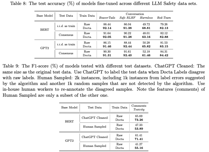
• After cleaning label errors and fine-tuning BERT and GPT2 on different datasets, the test scores show that the proposed algorithm (i.e., Docta) consistently improves the model performances despite the smaller sizes of the Docta training sets.

  

Miscellaneous Notes