Research Notes | Generalizable Hate Speech Detection

Overview

This post is the summary of the following methods; they rank top on the CivilComments-WILDS benchmark:

Rank Method Paper
1 FISH [2104.09937] Gradient Matching for Domain Generalization (Shi et al., ICLR 2022
2, 3 IRMX [2206.07766] Pareto Invariant Risk Minimization: Towards Mitigating the Optimization Dilemma in Out-of-Distribution Generalization (Chen et al., ICLR 2023)
4 LISA [2201.00299] Improving Out-of-Distribution Robustness via Selective Augmentation (Yao et al., ICML 2022)
5 DFR [2204.02937] Last Layer Re-Training is Sufficient for Robustness to Spurious Correlations (Kirichenko et al., ICLR 2023)
6, 8 Group DRO
7, 12 Reweighting [1901.05555] Class-Balanced Loss Based on Effective Number of Samples (Cui et al., CVPR 2019) is one example that uses this method; the reweighting method could date back to much earlier works.

Reweighting, IRM, and CORAL

IRM [2] and CORAL [3] are two extensions of the basic reweighting method by adding an additional penalty term on top of the reweighting loss; this term is based on some measures of the data representations from different domains to encourage the data distribution of different domains to be similar.

Reference

  1. [2012.07421] WILDS: A Benchmark of in-the-Wild Distribution Shifts
  2. [1907.02893] Invariant Risk Minimization (Arjovsky et al.)
  3. [2007.01434] In Search of Lost Domain Generalization (Gulrajani and Lopez-Paz)

Reading Notes | Wild-Time – A Benchmark of in-the-Wild Distribution Shift over Time

[Semantic Scholar] – [Code] – [Tweet] – [Video] – [Website and Leaderboard] – [Slide] – [Lead Author]

Change Logs:

  • 2023-10-03: First draft. The authors provide 5 datasets (2 of them are text classification datasets, the others include 2 image classification datasets and 1 EHR dataset) and more than 10 mitigation methods for distribution shift.

Experiments

  • The authors find that most of the mitigation methods are not effective compared to the standard ERM on the proposed benchmark. Note that SimCLR and SwaV methods are only applicable to image classification tasks.

    image-20231003120134331

image-20231003120318062

Additional Notes

From the content below, we could see that:

To address this challenge, we adapt the above invariant learning approaches to the temporal distribution shift setting. We leverage timestamp metadata to create a temporal robustness set consisting of substreams of data, where each substream is treated as one domain. Specifically, as shown in Figure 3, we define a sliding window G with length L. For a data stream with T timestamps, we apply the sliding window G to obtain T − L + 1 substreams. We treat each substream as a “domain” and apply the above invariant algorithms on the robustness set. We name the adapted CORAL, GroupDRO and IRM as CORAL-T, GroupDRO-T, IRM-T, respectively. Note that we do not adapt LISA since the intra-label LISA performs well without domain information, which is also mentioned in the original paper.

  • The way the authors apply the group algorithms look questionable: it does not make sense to create artificial domains by grouping data from some consecutive timestamps. This may be the reason why the authors do not observe the performance gains.
  • The LISA, which is the same author’s work, seems to be a good approach as it does not require the domain labels while performing competitively.

Reading Notes | Competency Problems – On Finding and Removing Artifacts in Language Data

[Semantic Scholar] – [Code] – [Tweet] – [Video] – [Website] – [Slide]

Change Logs:

  • 2023-09-26: First draft. The paper appears at EMNLP 2021.
  • The following is the main claim of the paper, as is summarized in [1]:

[…] all correlations between labels and individual “input features” are spurious.

  • Spurious correlation is useful in the training data but unreliable in general [1].

Reference

  1. Informativeness and Invariance: Two Perspectives on Spurious Correlations in Natural Language (Eisenstein, NAACL 2022): This paper updates the claim in the main paper theoretically: feature-label correlation is not related to whether label is invariant to the the interventions on the feature.

    Practically, the paper suggests the partial invariance (whether independent or not) for real-world datasets; for example, the sentiment of a movie review is invariant to the actor names. The paper also suggest the following options to improve model robustness:

    data augmentation, causally-motivated regularizers, stress tests, and “worst-subgroup” performance metrics (and associated robust optimizers) can be seen as enforcing or testing task-specific invariance properties that provide robustness against known distributional shifts (e.g., Lu et al., 2020; Ribeiro et al., 2020; Kaushik et al., 2021; Koh et al., 2021; Veitch et al., 2021). Such approaches generally require domain knowledge about the linguistic and causal properties of the task at hand — or to put it more positively, they make it possible for such domain knowledge to be brought to bear. Indeed, the central argument of this paper is that no meaningful definition of spuriousness or robustness can be obtained without such domain knowledge.

  2. On the Limitations of Dataset Balancing: The Lost Battle Against Spurious Correlations (Schwartz & Stanovsky, Findings 2022): This paper shows that creating a truly balanced dataset devoid of the issues mentioned in the main paper will also throw the useful signals encoded in the texts (“throw the baby out with the bathwater”).

Reading Notes | NoisywikiHow – A Benchmark for Learning with Real-world Noisy Labels in Natural Language Processing

[Semantic Scholar] – [Code] – [Tweet] – [Video] – [Website] – [Slide]

Change Logs:

  • 2023-09-14: First draft. The paper appears at ACL 2023. The code base has very detailed instructions on how to reproduce their results.

Method

  • The authors find that the labeling errors are both annotator-dependent and instance-dependent.

Experiments

  • The best performing LNL method on the benchmark is SEAL [1]: one could also consider MixUp regularization [2]. All other LNL methods have almost indistinguishable difference as the base models, i.e., not doing any intervention on the training process.

Additional Note

Comments

  • The reason why creating a new dataset is necessary is that the users could customize the noise level to compare performances of different algorithms in a controlled setting.

Reference

  1. [2012.05458] Beyond Class-Conditional Assumption: A Primary Attempt to Combat Instance-Dependent Label Noise (Chen et al. AAAI 2021).
  2. [1710.09412] mixup: Beyond Empirical Risk Minimization (Zhang et al., ICLR 2018, 7.6K citations).
  3. Nonlinear Mixup: Out-of-Manifold Data Augmentation for Text Classification (Guo, AAAI 2020). One application of MixUp regularization in NLP. It is based on a CNN classifier and the improvement is quite marginal.
  4. [2006.06049] On Mixup Regularization (Carratino et al., JMLR): A theoretical analysis of MixUp regularization.
  5. Learning with Noisy Labels (Natarajan et al., NIPS 2013): This paper is the first paper that (theoretically) studies LNL. It considers the binary classification problem where labels are randomly flipped, which is theoretically appealing but less relevant empirically according to the main paper.

Reading Notes | Improving Generalization of Hate Speech Detection Systems to Novel Target Groups via Domain Adaptation

[Semantic Scholar] – [Code] – [Tweet] – [Video] – [Website] – [Slide]

Change Logs:

  • 2023-09-11: First draft. This paper appears at WOAH ’22.

The paper studies the generalization to new hate target groups on the single HateXplain dataset; they authors do so by comparing three existing methods, including (1) Unsupervised Domain Adaptation (UDA, this method is also used in paper [1]), (2) MixUp regularization, (3) curriculum labeling, and (4) DANN.

The paper also considers the back translation approach (specifically (en, fr), (en, de), and (en, es)) for data augmentation.

Experiments

  • Zero: Directly apply a model trained on \mathcal{D}_A to a new domain \mathcal{D}_B.
  • Zero+: Augmenting \mathcal{D}_A using back-translation.
  • ZeroB+: Applying back-translation-based data augmentation while making sure that the each batch is class-balanced.

Reference

  1. Unsupervised Domain Adaptation in Cross-corpora Abusive Language Detection (Bose et al., SocialNLP 2021): This paper considers the setting of training on dataset \mathcal{D}_A and testing on another dataset \mathcal{D}_B, where A, B are HateEval, Waseem, and Davidson, resulting in 6 pairs. They use several existing methods to improve the test scores on \mathcal{D}_B.
  2. [2012.10289] HateXplain: A Benchmark Dataset for Explainable Hate Speech Detection (Mathew et al., AAAI 2021): This used to be the only dataset that provides the target groups of both hateful and non-hateful contents.
  3. d: Data augmentation could happen in symbol space via rules, word replacement through BERT, text-generation models or feature space. However, the main paper chooses to use the back translation for data augmentation.

    Here are two libraries on data augmentation in NLP:

Reading Notes | WILDS – A Benchmark of in-the-Wild Distribution Shifts

[Semantic Scholar] – [Code] – [Tweet] – [Video] – [Website] – [Slide] – [Leaderboard]

Change Logs:

  • 2023-09-06: First draft. The paper provides a standardized package for many domain generalization algorithms, including group DRO, DANN, and Coral.

Background

Distribution shifts happen when test conditions are “newer” or “smaller” compared to training conditions. The paper defines them as

  • Newer: Domain Generalization

    The test distribution is related to but distinct (aka. new or unseen during training) to the training distributions. Note that the test conditions are not necessarily a superset of the training conditions; they are not “larger” compared to the “smaller” case described below.

    Here are two typical examples of domain generalization described in the paper:

    • Training a model based on patient information from some hospitals and expect the model to generalize to many more hospitals; these hospitals may or may not be a superset of the hospitals we collect training data from.
    • Training an animal recognition model on images taken from some existing cameras and expect the model to work on images taken on the newer cameras.
  • Smaller: Subpopulation Shift

    The test distribution is a subpopulation of the training distributions. For example, degraded facial recognition accuracy on the underrepresented demographic groups ([3] and [4]).
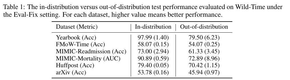
Evaluation

The goal of OOD generalization is training a model on data sampled from training distribution P^\text{train} that performs well on the test distribution P^\text{test}. Note that as we could not assume the data from two distributions are equally difficult to learn, the most ideal case is to at least train two models (or even more ideally three models) and take 2 (or 3) measurements:

Index Goal Training Data Testing Data
1 Measuring OOD Generalization $D ^ \text{train} \sim P^ \text{train}$ $D ^ \text{test} \sim P^ \text{test}$
2 Ruling Out Confounding Factor of Distribution Difficulty $D ^ \text{test} _ \text{heldout} \sim P^ \text{test}$ $D ^ \text{test} \sim P^ \text{test}$
3 (Optional) Sanity Check $D ^ \text{train} \sim P^ \text{train}$ $D ^ \text{train} _ \text{heldout} \sim P^ \text{train}$

However, the generally small test sets make the measurement 2 hard or even impossible: we could not find an additional held-out set D ^ \text{test} _ \text{heldout} that matches the size of D ^ \text{train} to train a model.

The authors therefore define 4 relaxed settings:

Index Setting Training Data Testing Data
1 Mixed-to-Test Mixture of P^ \text{train} and P^ \text{test} $P^ \text{train}$
2 Train-to-Train (aka. setting 3 above) $P^ \text{train}$ $P^ \text{train}$
3 Average. This is a special case of 2; it is only suitable for subpopulation shift, such as Amazon Reviews and CivilComments. Average Performance Worst-Group Performance
4 Random Split. This setting destroys the P ^ \text{test}. $\tilde{D} ^ \text{train} := \mathrm{Sample}(D ^ \text{train} \cup D ^ \text{test})$ $(D ^ \text{train} \cup D ^ \text{test}) \backslash \tilde{D} ^ \text{train}$

image-20231003161354088

Dataset

The dataset includes regular and medical image, graph, and text datasets; 3 out of 10 are text datasets, where the less familiar Py150 is a code completion dataset. Note that the authors fail to cleanly define why there are subpopulation shifts for Amazon Reviews and Py150 datasets as the authors acknowledge below:

However, it is not always possible to cleanly define a problem as one or the other; for example, a test domain might be present in the training set but at a very low frequency.

For Amazon Reviews dataset, one viable explanation on why there is subpopulation shift is uneven distribution of reviews on the same product in the train, validation, and test set.

Name Domain Generalization Subpopulation Shift Notes
CivilComments No; this is because the demographic information of the writers are unknown; if such information is known, we could also create a version with domain generation concern. Yes; this is because the mentions of 8 target demographic groups are available. The only dataset with only subpopulation shift.
Amazon Reviews Yes; due to disjoint users in the train, OOD validation, and OOD test set; there are also ID validation and ID test set from same users as the training set. Yes
Py150 Yes; due to disjoint repositories in train, OOD validation, and OOD test set; there are also ID validation and ID test set from same repositories as the training set. Yes

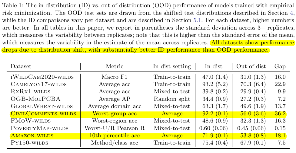
Importantly, the authors note that performance drop is a necessary condition of distribution shifts. That is

  • The presence of distribution shifts do not lead to performance drop on the test set.
  • If we observe degraded test set performance, then there might be distribution shifts (either domain generalization or subpopulation shift). Here are two examples:

    • Time Shift in Amazon Review Dataset: The model trained on 2000 – 2013 datasets perform similarly well (with 1.1% difference in F1) as the model trained on 2014 – 2018 datasets on the test set sampled from 2014 – 2018.
    • Time and User Shift in Yelp Dataset: For the time shift, the setting is similar as Amazon Reviews; the authors observe a maximum of 3.1% difference. For the user shift, whether the data splits are disjoint in terms of users only influence the scores very little.

Experiments

Here is a summary of the authors’ experiments. Note that Yelp is not the part of the official dataset because it shows no evidence for distribution shift.

Index Dataset Shift Existence
1 Amazon Reviews Time No
2 Amazon Reviews Category Maybe
3 CivilComments Subpopulation Yes
4 Yelp Time No
5 Yelp User No

Amazon Reviews

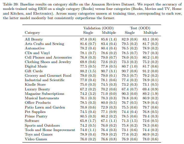
The authors train a model on one category (“Single”) and four categories (“Multiple”, “Multiple” is a superset of “Single”) and measure the test accuracy on other 23 disjoint categories.

The authors find that (1) training with more categories modestly yet consistently improves the scores, (2) the OOD category (for example, “All Beauty”) could have an even higher score than the ID categories, (3) the authors do not see strong evidence of domain shift as they could not rule out other confounding factors. Note that the authors here use the very vague term “intrinsic difficulty” to gloss over something they could not explain well.

While the accuracies on some unseen categories are lower than the train-to-train in-distribution accuracy, it is unclear whether the performance gaps stem from the distribution shift or differences in intrinsic difficulty across categories; in fact, the accuracy is higher on many unseen categories (e.g., All Beauty) than on the in-distribution categories, illustrating the importance of accounting for intrinsic difficulty.

To control for intrinsic difficulty, we ran a test-to-test comparison on each target category. We controlled for the number of training reviews to the extent possible; the standard model is trained on 1 million reviews in the official split, and each test-to-test model is trained on 1 million reviews or less, as limited by the number of reviews per category. We observed performance drops on some categories, for example on Clothing, Shoes, and Jewelry (83.0% in the test-to-test setting versus 75.2% in the official setting trained on the four different categories) and on Pet Supplies (78.8% to 76.8%). However, on the remaining categories, we observed more modest performance gaps, if at all. While we thus found no evidence for significance performance drops for many categories, these results do not rule out such drops either: one confounding factor is that some of the oracle models are trained on significantly smaller training sets and therefore underestimate the in-distribution performance.

image-20231002193306896

The authors also control the size consistent for “Single” and “Multiple” settings. They show that training data with more domains (with increased diversity) is beneficial for improving OOD accuracies.

CivilComments

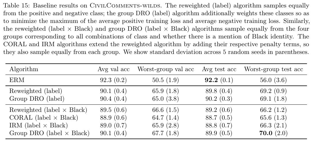
Each sample in the dataset has a piece of text, 1 binary toxicity labels, and 8 target labels (each text could include zero, one, or more identities). The authors use 8 TPR and TNR values to measure the performance (totaling 16 numbers).

The authors observe subpopulation shifts: despite 92.2% average accuracy, the worst number among 16 numbers is merely 57.4%. A comparison of 4 mitigation methods shows that (1) the group DRO has the best performance, (2) the reweighting baseline is quite strong, the improved versions of reweighting (i.e., CORAL and IRM) are likely less useful.

In light of the effectiveness of the group DRO algorithm, the authors extend the number of groups to 2 ^ 9= 512, the resulting performance does not improve.

image-20231002190304265

Additional Notes

  • Deciding Type of Distribution Shift

    As long as there are no clearly disjoint train, validation, and test set as in Amazon Reviews and Py150 datasets, then there is no domain generalization issue; presence of a few unseen users in the validation or test set should not be considered as the domain generalization case.

  • Challenge Sets vs. Distribution Shifts

    The CheckList-style challenge sets, such as HANS, PAWS, CheckList, and counterfactually-augmented datasets like [5], are intentionally created different from the training set.

Reference

  1. [2201.00299] Improving Out-of-Distribution Robustness via Selective Augmentation (Yao et al.): This paper proposes the LISA method that performs best on the Amazon dataset according to the leaderboard.
  2. [2104.09937] Gradient Matching for Domain Generalization (Shi et al.): This paper proposes the FISH method that performs best on the CivilComments dataset on the leaderboard.
  3. Gender Shades: Intersectional Accuracy Disparities in Commercial Gender Classification (Buolamwini and Gebru, FAccT ’18)
  4. Racial Disparities in Automated Speech Recognition (Koenecke et al., PNAS)
  5. [2010.02114] Explaining The Efficacy of Counterfactually Augmented Data (Kaushik et al., ICLR ’20)
  6. [2004.14444] The Effect of Natural Distribution Shift on Question Answering Models (Miller et al.): This paper trains 100+ QA models and tests them across different domains.
  7. Selective Question Answering under Domain Shift (Kamath et al., ACL 2020): This paper creates a test set of mixture of ID and OOD domains.

Reading Notes | Distributionally Robust Neural Networks for Group Shifts – On the Importance of Regularization for Worst-Case Generalization

[Semantic Scholar] – [Code] – [Tweet] – [Video] – [Website] – [Slide] – [HuggingFace]

Change Logs:

  • 2023-09-06: First draft. This paper appears at ICLR ’20.
  • 2023-09-07: Add the “example” section for easy visualization.

Background

ERM and DRO

  • ERM

    ERM tries to minimize the empirical risk. Here \hat{P} denotes the empirical distribution of the true underlying distribution P of training data.

\hat{\theta} _ \mathrm{ERM} := \mathbb{E} _ {(x, y) \sim \hat{P}} \left[ \ell((x, y); \theta)\right]

  • DRO

    DRO tries to find \theta that minimizes the worst-group risk \hat{\mathcal{R}}(\theta). The practical form of DRO is called group DRO (i.e., gDRO). See the application section on how the groups are defined.

\hat{\theta} _ \mathrm{DRO} := \arg\min _ \theta \left[ \hat{\mathcal{R}}(\theta):=\max _ {g \in \mathcal{G}}\mathbb{E} _ {(x, y) \sim \hat{P} _ g} \left[ \ell(x, y); \theta) \right] \right]

Example

To better visualize the strength of gDRO over ERM, we can look at a linear regression example; this example is taken from Stanford CS 221.

The objective of linear regression is Mean Square Error (MSE) \arg\min_{\mathbf{w}} (\mathbf{w}^T\mathbf{x} -y) ^ 2; fitting the entire datasets gives a much higher group A loss (i.e. 21.26) than group B loss (i.e. 0.31) even though the total loss is 7.29.

from sklearn.linear_model import LinearRegression
from sklearn.metrics import mean_squared_error

x = np.array([1, 2, 5, 6, 7, 8])[:, np.newaxis]
y = np.array([4, 8, 5, 6, 7, 8])

reg = LinearRegression(fit_intercept=False)
reg.fit(x, y)

print(mean_squared_error(reg.predict(x[:2]), y[:2]))
print(mean_squared_error(reg.predict(x[2:]), y[2:]))
print(mean_squared_error(reg.predict(x), y))

Note that the second plot shows how changing \mathbf{w} leads to differences in the loss over each group (yellow or blue) and the aggregated group (red). We can see that optimizing the aggregated loss leads to a solution that bias group B. However, if we optimize the pointwise maximum (purple), we could improve have a more reasonable curve.

image-20230907124813672

image-20230907123929901

Application

  • Mitigating Spurious Correlation

    In order to train a classifier that is not affected by spurious correlation, we can partition training dataset into groups with multiple attributes \mathcal{A} based on some prior knowledge and then form the group using \mathcal{A} \times \mathcal{Y}. For example, the paper [1] observes that negation spuriously correlates with the contradiction label. Therefore, one natural choice of \mathcal{A} is “texts with negation words” and “texts without negation words;” this will lead to m=2 \times 3 = 6 groups.

  • Improving Training on Data Mixture

    Training a classifier using a mixture of datasets \cup _ {k=1}^K \mathcal{D} _ k with the same label space \mathcal{Y}; this will give us K \times \vert \mathcal{Y}\vert groups. This is a more natural application of DRO as we have well-defined \mathcal{A} that does not depend on prior knowledge.

Method

For large discriminative models, neither ERM nor gDRO is able to attain a low worst-group test error due to a high worst-group generalization gap.

Model Method Training Error Worst-Group Test Error
Many Models ERM Low High
Small Convex Discriminative Model or Generative Model gDRO Low Low
Large Discriminative Model (e.g., ResNet or BERT) gDRO Low High

The authors propose to add simple regularization to gDRO to address the problem; they try \ell_2 regularization and early stopping. Even though these methods are frequently used approaches, it is a novel complement to the observations in influential work [4]: regularization may be necessary to make gDRO work for large discriminative models.

image-20230906211211382

Additional Note

  • Probability Simplex

    A probability simplex \Delta is a geometric representation of all probabilities of n events. If there are n events, then \Delta is a (n-1)-dimensional convex set that includes all possible n-dimensional probability vectors \mathbf{p}; it satisfies \mathbf{1}^T \mathbf{p}=1 with non-negative entries. The boundary of \Delta is determined by extreme one-hot probability vectors.

    The visualization of a probability simplex depicting 3 events is a triangular plane determined by three extreme points (1, 0, 0), (0, 1, 0), (0,0, 1).

  • Measures of Robustness

The paper uses the generalization on the worst-accuracy group as a proxy for robustness.

Reference

  1. Right for the Wrong Reasons: Diagnosing Syntactic Heuristics in Natural Language Inference (McCoy et al., ACL 2019): This paper identifies three shortcuts (called “heuristics” in the paper) that could be exploited by an NLI classifier: (1) lexical overlap, (2) subsequence, and (3) constituent. The authors also propose the famous HANS (Heuristic Analysis for NLI Systems) test set to diagnose the shortcut learning.

    Instead of using these cases to overrule the lexical overlap heuristic, a model might account for them by learning to assume that the label is contradiction whenever there is negation in the premise but not the hypothesis.

  2. Annotation Artifacts in Natural Language Inference Data (Gururangan et al., NAACL 2018): This paper shows that a significant portion of SNLI and MNLI test sets could be classified correctly without premises.
  3. [1806.08010] Fairness Without Demographics in Repeated Loss Minimization (Hashimoto et al.): The application of DRO in fair classification.
  4. [1611.03530] Understanding deep learning requires rethinking generalization (Zhang et al.; more than 5K citations): This paper makes two important observations and rules out the VC dimension, Rademacher complexity as possible explanations.

    • The neural network is able to attain zero training error for (1) a dataset with real images but random label, and (2) a dataset of random noise and random labels through memorization. The testing error is still near chance.
    • Because of the last bullet point, the regularization may not help with generalization at all; it is neither a necessary nor a sufficient condition to generalization.