[Semantic Scholar] – [Code] – [Tweet] – [Video] – [Website] – [Slide]
Change Logs:
- 2023-10-03: First draft.
Tag: DataSelection
Reading Notes | Exploring and Predicting Transferability across NLP Tasks
[Semantic Scholar] – [Code] – [Tweet] – [Video] – [Website] – [Slide]
Change Logs:
- 2023-09-16: First draft. This paper appears at ACL 2020.
- Data selection strategy for best transfer learning performance.
Reference
Reading Notes | Understanding Dataset Difficulty with V-Usable Information
[Semantic Scholar] – [Code] – [Tweet] – [Video] – [Website] – [Slide]
Change Logs:
- 2023-09-19: First draft. This paper appears as one of the outstanding papers at ICML 2022.
Overview
The main contribution of the paper is a metric to evaluate the difficulty of the aggregate and sample-wise difficulty of a dataset for a model family \mathcal{V}: a lower score indicates a more difficult dataset. This metric is appealing because it is able to do five things while previous approaches could only do 1 to 3 of them. Specifically,
- Comparing Datasets: DIME (accepted as a workshop paper at NeurIPS 2020), IRT [4].
- Comparing Models: Dynascore [3]
- Comparing Instances: Data Shapley [5]
- Comparing Dataset Slices
- Comparing Attributes: The paper [6] estimates the attribute importance using MDL.
Method
Despite a lot of theoretical construct in Section 2, the way to compute the proposed metric is indeed fairly straightforward.
Suppose we have a dataset \mathcal{D} _ \text{train} and \mathcal{D} _ \text{test} of a task, such as NLI, the proposed metric requires fine-tuning on \mathcal{D} _ \text{train} two models from the same base model \mathcal{V} and collecting measurements on \mathcal{D} _ \text{test} (Algorithm 1):
-
Step 1: Fine-tuning a model g’ on \mathcal{D} _ \text{train} = { (x_1, y_1), \cdots, (x_m, y_m) } and another model g on { (\phi, y_1), \cdots, (\phi, y_m) }, where \phi is an empty string; both g’ and g are the model initialized from the same base model, such as
bert-base-uncased. -
Step 2: For each test sample, the sample-wise difficulty (aka. PVI) is defined as \mathrm{PVI}(x_i \rightarrow y_i) := -\log_2 g(y_i\vert \phi) + \log_2 g'(y_i\vert x_i); the aggregate difficulty is its average \hat{I} _ \mathcal{V}(X \rightarrow Y) = \frac{1}{n}\sum _ i \mathrm{PVI}(x_i \rightarrow y_i).
If the input and output are independent, the metric is provably and 0; it will be empirically close to 0.
Note that:
- The method requires a reasonably large dataset \mathcal{D} _ \text{train}. However, the exact size is not known in advance unless we train many models and wait to see when the curve plateaus, which is not feasible in practice. The authors use 80% of the SNLI dataset for estimation (Appendix A).
- The specific choice of models, hyperparameters, and random initializations does not influence the results a lot (Section 3.2).
Applications
There are several applications when we use the proposed metric to rank the samples in a dataset:
- Identifying the annotation errors (Section 3).
- Using the metric to select challenging samples for data selection, including training data selection, data augmentation, and TCP (Section 4).
- Guiding the creation of new specifications as it is possible to compute the token-wise metric (Section 4.3).
Additional Notes
- It is quite surprising that the CoLA dataset is more difficult than SNLI and MNLI according to the authors’ measure.
Code
Reference
- Dataset Cartography: Mapping and Diagnosing Datasets with Training Dynamics (Swayamdipta et al., EMNLP 2020): The method in the main paper and this paper both requires training a model.
- [2002.10689] A Theory of Usable Information Under Computational Constraints (Xu et al., ICLR 2020).
- [2106.06052] Dynaboard: An Evaluation-As-A-Service Platform for Holistic Next-Generation Benchmarking
- Evaluation Examples are not Equally Informative: How should that change NLP Leaderboards? (Rodriguez et al., ACL-IJCNLP 2021)
- [1904.02868] Data Shapley: Equitable Valuation of Data for Machine Learning (ICML 2019): Data shapley could give a pointwise estimate of a sample’s contribution to the decision boundary.
- [2103.03872] Rissanen Data Analysis: Examining Dataset Characteristics via Description Length (ICML 2021).
Reading Notes | GIO – Gradient Information Optimization for Training Dataset Selection
[Semantic Scholar] – [Code] – [Tweet] – [Video] – [Website] – [Slide]
Change Logs:
- 2023-09-19: First draft.
Reference
Research Notes | Training Data Optimization
Problem Statement
Suppose we have a collection of datasets from K sources \mathcal{D} _ 1, \cdots, \mathcal{D} _ K. These K datasets have been unified regarding input and output spaces.
Now we split each \mathcal{D} _ i into train, validation, and test splits \mathcal{D} _ i ^ \text{train},\ \mathcal{D} _ i ^ \text{val} and \mathcal{D} _ i ^ \text{test} and form the aggregated train, validation, and test sets as \mathcal{D}^\text{train} := \cup _ {i=1}^ K D _ i^\text{train}, \mathcal{D}^\text{val} := \cup _ {i=1}^ K D _ i^\text{val}, and \mathcal{D}^\text{test} := \cup _ {i=1}^ K D _ i^\text{test} .
The learning problem could vary depending the quality of the datasets after (1) dataset collection and annotation by authors of different datasets, and (2) dataset unification when merging K datasets into one. This is because:
-
If labels are reliable, then this is dataset selection problem. The argument is to save computation resources when training on \mathcal{D} \subseteq \mathcal{D} ^ \text{train} while maintaining the performance as a model trained in (1) each \mathcal{D}_i,\ i \in [K], (2) \mathcal{D} ^ \text{train}, and (3) \mathrm{Sample}(\mathcal{D} ^ \text{train}) that matches the size of \mathcal{D}.
In some special cases, another motivation for dataset selection is that we know the size of a sampled dataset (for example, the dataset statistics described in a paper) but we are not sure what are exactly these samples.
- If labels are not reliable, then the argument is to prevent the low-quality labels from offsetting the benefits of a larger training dataset (rather than distilling a smaller dataset to save compute). We have three options:
| Index | Method | Type |
|---|---|---|
| 1 | Reannotating the entire dataset. This could be reduced as a dataset distillation problem as now we have more confidence on the filtered datasets. | Offline |
| 2 | Identifying and removing unreliable labels and optionally using these samples as an unsupervised dataset. This is also reducible to a dataset selection problem as 1. | Offline |
| 3 | Learning with the noisy labels (LNL as described in 1) they are; this requires the learning algorithm to explicitly consider the variablity in the label quality. | Online |
Note that there is a easily topic called “dataset distillation” that one may easily confused with. The goal of dataset distillation is to create synthetic dataset in the feature space based on the original one to match the performance on the test set. Previous show that it is possible to attain the original performance on MNIST ([3]) and IMDB ([4]) with a synthetic dataset of size (surprisingly) 10 and 20.
Adaptive Data Selection
With the test sets finalized, we could now work on sampling training sets, i.e., choosing one specific \mathrm{Sample}(\cdot) function described above. The goal here is to sample the training set so that the scores on the test sets are maximized:
- DSIR: Suppose we need to sample B batches of samples totaling K, then we could start by randomly sampling the 1st batch and then calling the DSIR algorithm in the future batches until we have collected K samples. This should be done for each label.
Reference
- NoisywikiHow: A Benchmark for Learning with Real-world Noisy Labels in Natural Language Processing (Wu et al., Findings 2023)
- [2202.01327] Adaptive Sampling Strategies to Construct Equitable Training Datasets (Cai et al., FAccT 2023)
- [2301.04272] Data Distillation: A Survey (Sachdeva and McAuley, JMLR).
- [1811.10959] Dataset Distillation (Wang et al.)
- [1910.02551] Soft-Label Dataset Distillation and Text Dataset Distillation (Sucholutsky and Schonlau, IJCNN 2020). This is the only paper referenced in 3 describing the dataset distillation for texts. This paper is based on the very original data distillation objective proposed in 4.
- [2302.03169] Data Selection for Language Models via Importance Resampling (Xie et al.)
- [2305.10429] DoReMi: Optimizing Data Mixtures Speeds Up Language Model Pretraining (Xie et al.)
-
[2306.11670] GIO: Gradient Information Optimization for Training Dataset Selection (Everaert and Potts): This paper has similar settings as the DSIR paper [6]: we are selecting new samples by minimizing their KL divergence with an existing set of unlabeled samples. The paper claims an advantage over the DSIR as the proposed algorithm requires fewer samples:
Like GIO, these heuristic methods aim to select a subset of data that is higher quality and more relevant. However, they are either highly tailored to their particular tasks or they require very large numbers of examples (to develop classifiers or construct target probabilities). By contrast, GIO is task- and domain-agnostic, it can be applied plug-and-play to a new task and dataset, and it requires comparatively few gold examples X to serve as the target distribution.
Reading Notes | Robust Hate Speech Detection in Social Media – A Cross-Dataset Empirical Evaluation
[Semantic Scholar] – [Code] – [Tweet] – [Video] – [Website] – [Slide] – [HuggingFace]
Change Logs:
- 2023-09-04: First draft. This paper appears at WOAH ’23. The provided models on HuggingFace have more than 40K downloads thanks to their easy-to-use
tweetnlppackage; the best-performing binary and multi-class classification models arecardiffnlp/twitter-roberta-base-hate-latestandcardiffnlp/twitter-roberta-base-hate-multiclass-latestrespectively.
Method
Datasets
The authors manually select and unify 13 hate speech datasets for binary and multi-class classification settings. The authors do not provide the rationale on why they choose these 13 datasets.
For the multi-class classification setting, the authors devise 7 classes: racism, sexism, disability, sexual orientation, religion, other, and non-hate. This category is similar to yet smaller than the MHS dataset, including gender, race, sexuality, religion, origin, politics, age, and disability (see [1]).
For all 13 datasets, the authors apply a 7:1:2 ratio of data splitting; they also create a small external test set (i.e., Indep). With test sets kept untouched, the authors consider 3 ways of preparing data:
- Training on the single dataset.
- Training on an aggregation of 13 datasets.
- Training on a sampled dataset from the aggregation in 2. Specifically, the authors (1) find the dataset size that leads to the highest score in 1, (2) sample the dataset proportionally by the each of 13 datasets’ sizes and the the ratio of hate versus non-hate to exactly 1:1.
The processed datasets are not provided by the authors. We need to follow the guides below to obtain them; the index of the datasets is kept consistent with the HuggingFace model hub and and main paper’s Table 1.
| Index | Dataset Name | Source | Notes |
|---|---|---|---|
| 1 | HatE | Link that requires filling in a Google form. | |
| 2 | MHS | ucberkeley-dlab/measuring-hate-speech |
|
| 3 | DEAP | Zenodo | |
| 4 | CMS | Link that requires registration and email verification. | |
| 5 | Offense | Link; this dataset is also called OLID. | |
| 6 | HateX | hatexplain and GitHub |
|
| 7 | LSC | GitHub | Dehydrated |
| 8 | MMHS | nedjmaou/MLMA_hate_speech and GitHub |
|
| 9 | HASOC | Link that requires uploading a signed agreement; this agreement takes up to 15 days to approve. | Not Available |
| 10 | AYR | GitHub | Dehydrated |
| 11 | AHSD | GitHub | |
| 12 | HTPO | Link | |
| 13 | HSHP | GitHub | Dehydrated |
The following are the papers that correspond to the list of datasets:
- SemEval-2019 Task 5: Multilingual Detection of Hate Speech Against Immigrants and Women in Twitter (Basile et al., SemEval 2019)
- The Measuring Hate Speech Corpus: Leveraging Rasch Measurement Theory for Data Perspectivism (Sachdeva et al., NLPerspectives 2022)
- Detecting East Asian Prejudice on Social Media (Vidgen et al., ALW 2020)
- [2004.12764] “Call me sexist, but…”: Revisiting Sexism Detection Using Psychological Scales and Adversarial Samples (Samory et al.)
- Predicting the Type and Target of Offensive Posts in Social Media (Zampieri et al., NAACL 2019)
- [2012.10289] HateXplain: A Benchmark Dataset for Explainable Hate Speech Detection (Mathew et al.)
- [1802.00393] Large Scale Crowdsourcing and Characterization of Twitter Abusive Behavior (Founta et al.)
- Multilingual and Multi-Aspect Hate Speech Analysis (Ousidhoum et al., EMNLP-IJCNLP 2019)
- [2108.05927] Overview of the HASOC track at FIRE 2020: Hate Speech and Offensive Content Identification in Indo-European Languages (Mandal et al.)
- Are You a Racist or Am I Seeing Things? Annotator Influence on Hate Speech Detection on Twitter (Waseem, NLP+CSS 2016)
- [1703.04009] Automated Hate Speech Detection and the Problem of Offensive Language (Davidson et al.)
- Hate Towards the Political Opponent: A Twitter Corpus Study of the 2020 US Elections on the Basis of Offensive Speech and Stance Detection (Grimminger & Klinger, WASSA 2021)
- Hateful Symbols or Hateful People? Predictive Features for Hate Speech Detection on Twitter (Waseem & Hovy, NAACL 2016)
Despite the availability of the sources, it is quite hard to reproduce the original dataset as (1) many of the datasets in the table do not come with the predefiend splits; the only datasets that are available and have such splits are HatE, HatX, and HTPO, (2) how the authors unify (for example, deriving binary label from potentially complicated provided labels) the datasets is unknown, and (3) how the authors process the texts is also unknown.
It is better to find a model whose checkpoints and exact training datasets are both available; one such example is the Alpaca language model.
Models and Fine-Tuning
The authors start from the bert-base-uncased, roberta-base, and two models specifically customized to Twitter (see [2], [3]). The authors carry out the HPO on learning rates, warmup rates, number of epochs, and batch size using hyperopt.
Experiments
-
The data preparation method 3 (
All*) performs better than the method 1 (MHS,AYR, etc). It also achieves the highest scores on theIndeptest set (Table 3).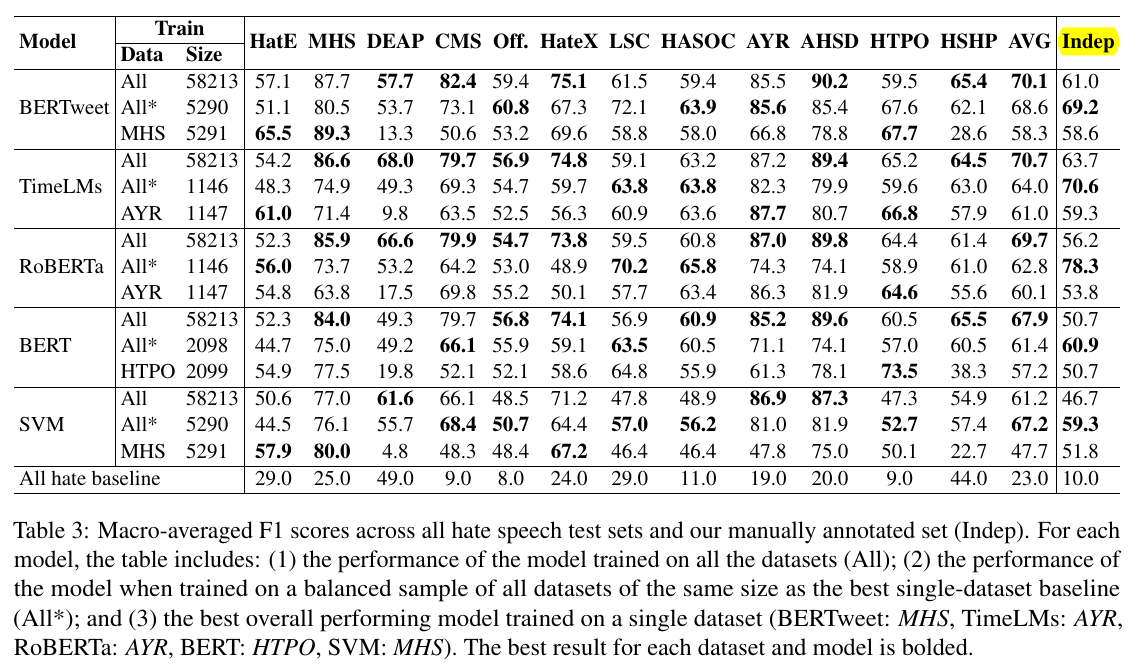
Other Information
- Language classification tasks could be done with
fasttextmodels (doc).
Comments
-
Ill-Defined Data Collection Goal
We can read the sentence like following from the paper:
- For example both CMS and AYR datasets deal with sexism but the models trained only on CMS perform poorly when evaluated on AYR (e.g. BERTweetCSM achieves 87% F1 on CSM, but only 52% on AYR).
- This may be due to the scope of the dataset, dealing with East Asian Prejudice during the COVID-19 pandemic, which is probably not well captured in the rest of the datasets.
The issue is that there is not quantitative measure of the underlying theme of a dataset (for example, CMS and AYR). The dataset curators may have some general ideas on what the dataset should be about; they often do not have a clearly defined measure to quantify how much one sample aligns with their data collection goals.
I wish to see some quantitative measures on topics and distributions of an NLP dataset.
Reference
- Targeted Identity Group Prediction in Hate Speech Corpora (Sachdeva et al., WOAH 2022)
- BERTweet: A pre-trained language model for English Tweets (Nguyen et al., EMNLP 2020)
- TimeLMs: Diachronic Language Models from Twitter (Loureiro et al., ACL 2022): This paper also comes from Cardiff NLP. It considers the time axis of the language modeling through continual learning. It tries to achieve OOD generalization (in terms of time) without degrading the performance on the static benchmark.
Reading Notes | DoReMi – Optimizing Data Mixtures Speeds Up Language Model Pretraining
Overview
Other Information
- The ratios of domains should be counted using number of tokens rather than number of documents, even though different tokenizers may return slightly different ratios.
Reference
- [2110.10372] Distributionally Robust Classifiers in Sentiment Analysis (Stanford Course Project Report).
-
Distributionally Robust Finetuning BERT for Covariate Drift in Spoken Language Understanding (Broscheit et al., ACL 2022): This paper is one of few papers I could find that applies DRO to an NLP model; the problem the authors addressing here is mitigating the spurious correlation (or improving robustness) of a cascade of text and token classification models.
The standard ERM (aka. MLE) assumes a single distribution and therefore all losses are equally important. However, the DRO tries to minimize the maximum (i.e., the worse case) of a set of distributions; this set of distributions is modeled by prior knowledge.
- [1810.08750] Learning Models with Uniform Performance via Distributionally Robust Optimization
-
Distributionally Robust Language Modeling (Oren et al., EMNLP-IJCNLP 2019): The main paper extensively cites this paper. The goal of this paper is to train a language model on a dataset mixture of K sources \cup _ {i=1}^K\mathcal{D} _ i without degrading the perform on each domain’s test set; it is a practical application of [3] in language modeling.
This setting may be useful because (1) each \mathcal{D} _ i may not be large enough to train the model, and (2) the authors observe that training on data mixture degrades the performance on the each domain’s test set than using a smaller dataset.
- [1911.08731] Distributionally Robust Neural Networks for Group Shifts: On the Importance of Regularization for Worst-Case Generalization (ICLR ’20; 1K citations). This paper fine-tunes BERT using DRO on the MNLI dataset; the paper also experiments on the image datasets.