Contents
Overview
The following notes are the data-centric AI IAP course notes from MIT; Independent Activities Period (IAP) is a special four-week semester of MIT. The standard time for each lecture is 1 hour.
Lecture 1 – Data-Centric AI vs. Model-Centric AI
-
It is not hard to design fancy models and apply various tricks on the well curated data. However, these models and tricks do not work for real-world data if we do not explicitly consider the real-world complexities and take them into account. Therefore, it is important to focus on data rather than model.
It turns out there are pervasive label errors on the most cited test sets of different modalities, including text, image, and audio. They could be explored in
labelerrors.com. - To understand why data is important, we could think about kNN algorithm. The accuracy of kNN is purely based on the quality of datasets. However, the kNN is not a data-centric algorithm because it does not modify the labels.
-
Two Goals of Data-Centric AI
Rather than modifying loss function, doing HPO, or changing the model itself, we do either of the following:
- Designing an algorithm that tries to understand the data and using that information to improve the model. One such example is curriculum learning by Yoshua Bengio; in curriculum learning, the data is not changed but its order is shuffled.
- Modifying the dataset itself to improve the models. For example, the confident learning (i.e., removing wrong labels before training the model) studied by Curtis Northcutt.
-
What are NOT Data-Centric AI and Data-Centric AI Counterpart
- Hand-picking data points you think you will improve a model. \rightarrow Coreset Selection.
- Doubling the size of dataset. \rightarrow Data Augmentation. For example, back-translation for texts, rotation and cropping for images. However, we need to first fix label errors before augmenting the data.
-
Typical Examples of Data-Centric AI
Curtis Northcutt cites Andrew Ng and other sources on the importance of data in machine learning ([1] through [3]). Here are some examples of data-centric AI:
- Outlier Detection and Removal. However, this process relies on a validation process on which threshold to choose.
- Label Error Detection and Correction
- Data Augmentation
- Feature Engineering and Selection. For example, solving XOR problem by adding a new column.
- Establishing Consensus Labels during Crowd-sourcing.
- Active Learning. I want to improve 5% accuracy on the test set but I could afford as little new annotated data as possible.
- Curriculum Learning.
-
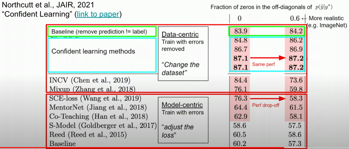
Data-Centric AI Algorithms are Often Superior to Model-Centric Algorithms
The model centric approaches (i.e., training less on what a model believes are the bad subset of data) is a much worse idea than the data-centric approach (i.e., confident learning).
- Root-Causing the Issues – Models or Data
- The model should perform well on the slices of data. Slicing means not only sampling data to a smaller number but also reducing the number of classes from a large number to a very small number. For example, rather than classifying images to 1000 classes, we only focus on performance on two classes.
- The model should perform similarly on similar datasets (for example, MNIST datasets and other digits dataset).
Lecture 2 – Label Errors
Notation
| Notation | Meaning | Note |
|---|---|---|
| $\tilde{y}$ | Noisy observed label | |
| $y ^ *$ | True underlying label | |
| $\mathbf{X} _ {\tilde{y} =i, y ^ {*} = j}$ | A set of examples whose true label is j but they are mislabeled as i. | |
| $\mathbf{C} _ {\tilde{y} =i, y ^ {*} = j}$ | The size of the dataset above. | |
| $p(\tilde{y} =i, y ^ {*} = j)$ | The joint probability of label i and label j; it could be estimated by normalizing \mathbf{C}; it is indeed dividing each entry by the sum of all entries in the matrix \mathbf{X}. | |
| $p(\tilde{y} =i\vert y ^ {*} = j)$ | The transition probability that the label j flips to label i; it could also be called flipping rate. |
Categories of Label Errors
When comparing the consensus crowd-sourcing labels and the final label in the dataset, there are 4 types of label errors:
- Correctable: The given label is wrong and it could be corrected with crowd-sourcing. This is the type of label the lecture focus on detecting.
- Multi-label: The given label and the consensus label are both right. However, more than one label in \mathcal{Y} could be used to label the samples. For example, an image with co-existence of laptop and humans that is incorrectly labeled as “laptop.”
- Neither: The given label and the consensus label are both wrong.
- Non-agreement: There is no way to tell whether the given label or the consensus label is correct.
There are also two categories of the label errors the presenter does not focus on:
- Uniform Random Flipping p(\hat{y} = i \vert y ^ * = j) = \epsilon, \forall i\neq j: This will show as a symmetric \mathbf{X} matrix. It is easy to solve and this type of errors are unlikely to happen in the real world.
- Instance-Dependent Label Noise p(\hat{y} = i \vert y ^ * = j, \mathbf{x}): This will require a lot of assumptions on the data distribution. Importantly, this type of label errors seldom happen in the real world.
Uncertainty
There are two sources of uncertainty:
- Aleatoric Uncertainty: Label noise. It is the difficulty of an sample. This difficulty could come from incorrect label y or the strange distribution of \mathbf{x}.
- Epistemic Uncertainty: Model noise. It is the model’s inability to understand the example. For example, the model has never seen similar examples before or the model class is too simple.
Confident Learning
The focus of the lecture is the correctable errors; it is defined in previous sections; the matrix \mathbf{X} is non-symmetric. Furthermore, the lecture will focus on samples with one label and one annotation.
-
Motivation of Using Confident Learning
- Ranking samples by loss does not work. We could not find a loss threshold and claim the samples above this threshold are label errors.
- Deep learning does not solve the label noise problem (despite many papers and many claims) because these problems try to solve the datasets polluted by uniform noise.
-
Assumption: Class-Conditional Label Noise
p(\hat{y} \vert y ^ {_}; \mathbf{x} ) = p(\hat{y} \vert y ^ {_})- Interpretation: Given the true label, there is a constant flipping rate for the samples under that true label to other labels.
- Rationale: A pig image often confused with a boar image but not other items such as “missiles” and “keyboards.” This tendency has nothing to do with what exactly a pig look like in an image but the similarities of the classes.
- Motivation: This assumption is made because the LHS couples the aleatoric uncertainy and epistemic uncertainty and this assumption decouples these two uncertainties.
-
Confident Learning
- For each of the class j, we could define a model’s self-confidence. If the self-confidence score of class j is low, but some of the samples have very high confidence, then we could say that there is something wrong with that label.
t _ j = \frac{1}{ \vert \mathbf{X} _ {\tilde{y} = j}\vert } \sum _ {x \in \mathbf{X} _ {\tilde{y} = j}} \hat{p} ( \tilde{y} = j; \mathbf{x}, \theta)
-
For samples labeled with i, if its predicted probability for class j larger then t _ j, then this sample is likely mislabeled and we could assign it to the set. We could obtain this matrix in a cross-validation style. For example, if we have 3 folds, we use 2/3 of the data to train the model \hat{p} and use the remaining 1/3 to compute this matrix.
\hat{ \mathbf{X} } _ {\tilde{y} = i, y ^ {*} = j} = { \mathbf{x} \in \mathbf{X} _ {\tilde{y} = i}: \hat{p} (\tilde{y} = j; \mathbf{x}, \theta) \geq t_j} -
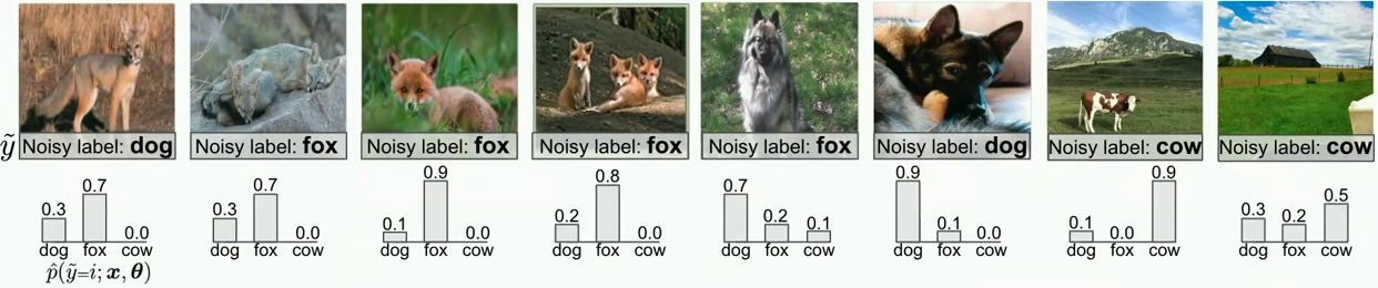
Example
Suppose we know the t _ j for “dog”, “fox”, and “cow” are 0.7, 0.7, and 0.9. We have following predictions and labels. We could obtain a matrix that looks like one below. The off-diagonal entries correspond to labeling errors.
$y ^ {*} = \text{dog}$ $y ^ {*} = \text{fox}$ $y ^ {*} = \text{cow}$ $\hat{y} = \text{dog}$ 1 1 0 $\hat{y} = \text{fox}$ 1 3 0 $\hat{y} = \text{cow}$ 0 0 1 Note the following:
- The last sample does not contain any animal and it is not counted. This shows that this scheme is robust to outliers.
- It is possible t _ j is very small but this will happen when there are many classes. In this case, the predicted probability for each class will also small.
-
Applications
-
Confident Learning + Ranking by Loss
If we see there are in total k off-diagonal samples, then we could pick the top-k samples based on loss values.
-
Confident Learning + Ranking by Normalized Margin
We could also rank by normalized margin for a specific class i; normalized margin is defined as following
p(\tilde{y} = i) – \max _ {j\neq i} p(\tilde{y} =j; \mathbf{x} \in \mathbf{X} _ i) -
Self-Confidence
When p(\tilde{y}=i) is close to 1, then as far as the model could think, the sample is not likely to be a label error.
-
Confident Learning + Ranking by Loss
Theory of Confident Learning
- The model-centric approaches (i.e., model reweighting methods) will still propagate the errors back to the weights. However, the data-centric approaches (i.e., pruning methods) does not have this problem.
- We could prove that even if the model is miscalibrated (i.e., overly confident in some classes), the confident learning method is still robust.
Implications on Testing
- When focusing on the subset of data whose labels could be corrected, more capable models (for example, ResNet-50 vs. ResNet-18) perform worse as they fit the random noise in the training set.
Lecture 8 – Encoding Human Priors
Human priors could be encoded (i.e., finding a function to represent) into the ML pipeline in two ways. During training time, it could be done using data augmentation. During test time, this is done through prompt engineering with an LLM.
- Data Augmentation
- Images: Flip, Rotation, Mobius transformation, Mixup. Mixup could be thought of as the linear interpolation of two images.
- Texts: Back-translation.
cleanlab Library
Anatomy
-
Understanding Cross-Validation in
cleanlabThe cross-validation in
cleanlabmeans the probabilities have to be the test scores. Specifically, if we have 3 folds, then what we will keep are the test prediction probabilities of each 1/3 fold using the model trained on the remaining 2/3 folds.This logic could be found in
estimate_confident_joint_and_cv_pred_proba()incleanlab/count.py; it is the most important functions forcleanlab. It is used infind_label_issuesfunction inCleanLearningclass; this class also inherits fromsklearn.base.BaseEstimator. The code could be found here. -
kerasis Necessary to Portcleanlabandtransformercleanlabrequires an API that similar tosklearn.- As of 2023-11-08, neither
transformerorsklearnteam provides a solution to port each other (except a less relevant library calledskopsthat is about sharingsklearnmodels to HuggingFace hub; also see news). We therefore need to rely thekeras-based code fromcleanlabofficial tutorial that fine-tunes a TF-basedbert-base-uncasedto find label errors inimdbdataset. - The complete script is available here.
Example
In the official demo that tries to find label errors in the imdb dataset, the authors use a simple MLP as the base model. The following (confusing at the first look) code indeed tokenize the texts into fixed length vectors (i.e., sequence_length).
import re
import string

import tensorflow as tf
import tensorflow_datasets as tfds
from tensorflow.keras.layers import TextVectorization

raw_train_ds = tfds.load(name="imdb_reviews", split="train", batch_size=-1, as_supervised=True)
raw_test_ds = tfds.load(name="imdb_reviews", split="test", batch_size=-1, as_supervised=True)

raw_train_texts, train_labels = tfds.as_numpy(raw_train_ds)
raw_test_texts, test_labels = tfds.as_numpy(raw_test_ds)

max_features = 10000
sequence_length = 250

def preprocess_text(input_data):
    lowercase = tf.strings.lower(input_data)
    stripped_html = tf.strings.regex_replace(lowercase, "
", " ")
    return tf.strings.regex_replace(stripped_html, f"[{re.escape(string.punctuation)}]", "")

vectorize_layer = TextVectorization(
    standardize=preprocess_text,
    max_tokens=max_features,
    output_mode="int",
    output_sequence_length=sequence_length,
)

vectorize_layer.reset_state()
vectorize_layer.adapt(raw_train_texts)

# (N, sequence_length)
train_texts = vectorize_layer(raw_train_texts).numpy()
test_texts = vectorize_layer(raw_test_texts).numpy()
Additional Notes
- “You are what you eat” is particularly relevant to the process of training machine learning models.
- The data collection, labeling, and cleaning process could be called “data engine” or “data flywheel” in tech firms (blog).
- The benefits of data-centric AI is that it disentangle the effects of data and modeling. Previously, we blindly trust the labels and efforts (including using larger models, changing loss functions, doing HPO) to improve the performance may only end up fitting the noise. If we make the data clean, we could identify what are the truly useful techniques and what are not.
-
cleanlabcould not only flag the label issues but also automatically fix the top label issues. (blog).Here we use Cleanlab Studio’s Clean Top K feature, which allows us to automatically correct the top most severe issues detected in our dataset with an automatically suggested label (inferred to be more suitable for each example than its original label in the dataset).
Reference
- Why it’s time for ‘data-centric artificial intelligence’ | MIT Sloan
- Bad Data Costs the U.S. $3 Trillion Per Year (Harvard Business Review)
- Bad Data: The $3 Trillion-Per-Year Problem That’s Actually Solvable | Entrepreneur
- [1710.09412] mixup: Beyond Empirical Risk Minimization (Zhang et al., ICLR 2017)