[Semantic Scholar] – [Code] – [Tweet] – [Video] – [Website] – [Slide]
Change Logs:
- 2023-08-28: First draft. This paper is a preprint even though it uses the ICML template.
Method
This paper tries to patch the frequently used Mahalanobis Distance (MD) OOD detection metric for image classification tasks. The issue with the MD metric is that it fails for near-OOD scenario [3]. For example, separating examples from CIFAR-10 and CIFAR-100. The authors also try to argue this using eigen analysis.
Suppose we have a classification dataset of K classes \mathcal{D} = \cup_{k=1}^K \mathcal{D}_k, then we fit K+1 MD on each \mathcal{D}_k\ (k=1, \cdots, K) and \mathcal{D}, then for a test sample \mathbf{x}, a higher score below shows that it is more likely to be an OOD sample:
\mathrm{RMD}_ k(\mathbf{x}) = \mathrm{MD}_ k(\mathbf{x}) – \mathrm{MD}_ 0(\mathbf{x}),\quad
\mathrm{OODScore}(\mathbf{x}) = \min_ k \mathrm{RMD}_ k(\mathbf{x})
Experiments
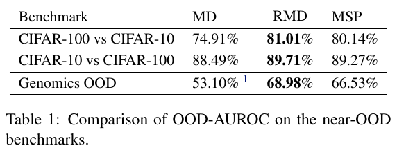
- The OOD detection performance is (1) asymmetrical, and (2) RMD does not significantly outperform MSP (Table 1).
Reference
-
A Simple Unified Framework for Detecting Out-of-Distribution Samples and Adversarial Attacks (NIPS ’18; 1.4K citations): This paper notes that the NNs tend to provide overly confident posterior distributions for OOD samples; this observation motivates the authors to propose the MD metric for OOD detection. The paper also draws the distinction between the adversarial samples and OOD samples.
-
[1610.02136] A Baseline for Detecting Misclassified and Out-of-Distribution Examples in Neural Networks (ICLR ’17): This is the paper that tries to detect OOD samples using posterior distribution \arg\max_{k=1,\cdots, K} p(k\vert \mathbf{x}). The paper [1] improves upon it.
-
[2007.05566] Contrastive Training for Improved Out-of-Distribution Detection: This paper strongly argues that the an OOD detection metric should work across the difficulty levels of detection tasks. Their proposed approach makes their metric more uniform. They propose the Confusion Log Probability (CLM) to measure the task difficulty. Specifically, they assume they have access to ID and OOD datasets \mathcal{D}_ \mathrm{in} and \mathcal{D}_ \mathrm{out} during training. Then,
-
Step 1: Training an ensemble of N_e classifiers on the union dataset \mathcal{D}_ \mathrm{in} \cup \mathcal{D}_ \mathrm{out}. Note that (1) the label space of these two datasets \mathcal{C}_ \text{in} and \mathcal{C}_ \text{out} are not necessarily same, (2) they need to hold out a test set \mathcal{D}_ \text{test} for Step 2, and (3) training a model ensemble is necessary for model calibration purposes (paper).
-
Step 2: Computing the CLM score as follows. A higher CLM score indicates that the domains of \mathcal{D}_ \text{in} and \mathcal{D}_ \text{out} are closer.
$$
\log\left( \frac{1}{\mathcal{D}_ {\vert\text{test}\vert}} \sum_{\mathbf{x} \in \mathcal{D}_ \text{test}} \sum_{k \in \mathcal{C}_ \text{in}} \frac{1}{N_e}\sum_{j=1}^{N_e} \mathcal{M}_ j(\mathbf{x}) \right)
$$