Reading Notes | DoReMi – Optimizing Data Mixtures Speeds Up Language Model Pretraining

Overview

Other Information

  • The ratios of domains should be counted using number of tokens rather than number of documents, even though different tokenizers may return slightly different ratios.

Reference

  1. [2110.10372] Distributionally Robust Classifiers in Sentiment Analysis (Stanford Course Project Report).
  2. Distributionally Robust Finetuning BERT for Covariate Drift in Spoken Language Understanding (Broscheit et al., ACL 2022): This paper is one of few papers I could find that applies DRO to an NLP model; the problem the authors addressing here is mitigating the spurious correlation (or improving robustness) of a cascade of text and token classification models.

    The standard ERM (aka. MLE) assumes a single distribution and therefore all losses are equally important. However, the DRO tries to minimize the maximum (i.e., the worse case) of a set of distributions; this set of distributions is modeled by prior knowledge.

  3. [1810.08750] Learning Models with Uniform Performance via Distributionally Robust Optimization
  4. Distributionally Robust Language Modeling (Oren et al., EMNLP-IJCNLP 2019): The main paper extensively cites this paper. The goal of this paper is to train a language model on a dataset mixture of K sources \cup _ {i=1}^K\mathcal{D} _ i without degrading the perform on each domain’s test set; it is a practical application of [3] in language modeling.

    This setting may be useful because (1) each \mathcal{D} _ i may not be large enough to train the model, and (2) the authors observe that training on data mixture degrades the performance on the each domain’s test set than using a smaller dataset.

  5. [1911.08731] Distributionally Robust Neural Networks for Group Shifts: On the Importance of Regularization for Worst-Case Generalization (ICLR ’20; 1K citations). This paper fine-tunes BERT using DRO on the MNLI dataset; the paper also experiments on the image datasets.

Reading Notes | Test Case Prioritization: An Empirical Study

Notes

[Semantic Scholar]- [Code] – [Tweet] – [Video] – [Website] – [Slide]

Change Logs:

  • 2023-08-27: First draft. This paper appeared at ICSM ’99. This conference was renamed to ICSME in 2014.
  • Test Case Prioritization (TCP) tries to order the test cases to optimize some objective, such as maximizing failure rates given a test budget of K or minimizing costs to obtain a coverage of \alpha.

  • TCP typically happens for regression testing, where we reuse the test suites and these test suites have historical statistics, such as actual failure rates on tests, coverage of branches or statements, and an estimation of probability of inducing bugs based on mutation.

Reading Notes | A Simple Fix to Mahalanobis Distance for Improving Near-OOD Detection

[Semantic Scholar] – [Code] – [Tweet] – [Video] – [Website] – [Slide]

Change Logs:

  • 2023-08-28: First draft. This paper is a preprint even though it uses the ICML template.

Method

This paper tries to patch the frequently used Mahalanobis Distance (MD) OOD detection metric for image classification tasks. The issue with the MD metric is that it fails for near-OOD scenario [3]. For example, separating examples from CIFAR-10 and CIFAR-100. The authors also try to argue this using eigen analysis.

Suppose we have a classification dataset of K classes \mathcal{D} = \cup_{k=1}^K \mathcal{D}_k, then we fit K+1 MD on each \mathcal{D}_k\ (k=1, \cdots, K) and \mathcal{D}, then for a test sample \mathbf{x}, a higher score below shows that it is more likely to be an OOD sample:

\mathrm{RMD}_ k(\mathbf{x}) = \mathrm{MD}_ k(\mathbf{x}) – \mathrm{MD}_ 0(\mathbf{x}),\quad
\mathrm{OODScore}(\mathbf{x}) = \min_ k \mathrm{RMD}_ k(\mathbf{x})

Experiments

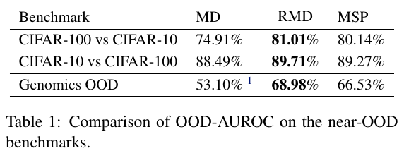
  • The OOD detection performance is (1) asymmetrical, and (2) RMD does not significantly outperform MSP (Table 1).

    image-20230828124958624

Reference

  1. A Simple Unified Framework for Detecting Out-of-Distribution Samples and Adversarial Attacks (NIPS ’18; 1.4K citations): This paper notes that the NNs tend to provide overly confident posterior distributions for OOD samples; this observation motivates the authors to propose the MD metric for OOD detection. The paper also draws the distinction between the adversarial samples and OOD samples.

  2. [1610.02136] A Baseline for Detecting Misclassified and Out-of-Distribution Examples in Neural Networks (ICLR ’17): This is the paper that tries to detect OOD samples using posterior distribution \arg\max_{k=1,\cdots, K} p(k\vert \mathbf{x}). The paper [1] improves upon it.

  3. [2007.05566] Contrastive Training for Improved Out-of-Distribution Detection: This paper strongly argues that the an OOD detection metric should work across the difficulty levels of detection tasks. Their proposed approach makes their metric more uniform. They propose the Confusion Log Probability (CLM) to measure the task difficulty. Specifically, they assume they have access to ID and OOD datasets \mathcal{D}_ \mathrm{in} and \mathcal{D}_ \mathrm{out} during training. Then,

  • Step 1: Training an ensemble of N_e classifiers on the union dataset \mathcal{D}_ \mathrm{in} \cup \mathcal{D}_ \mathrm{out}. Note that (1) the label space of these two datasets \mathcal{C}_ \text{in} and \mathcal{C}_ \text{out} are not necessarily same, (2) they need to hold out a test set \mathcal{D}_ \text{test} for Step 2, and (3) training a model ensemble is necessary for model calibration purposes (paper).

  • Step 2: Computing the CLM score as follows. A higher CLM score indicates that the domains of \mathcal{D}_ \text{in} and \mathcal{D}_ \text{out} are closer.

    $$
    \log\left( \frac{1}{\mathcal{D}_ {\vert\text{test}\vert}} \sum_{\mathbf{x} \in \mathcal{D}_ \text{test}} \sum_{k \in \mathcal{C}_ \text{in}} \frac{1}{N_e}\sum_{j=1}^{N_e} \mathcal{M}_ j(\mathbf{x}) \right)
    $$

Reading Notes | DeepGini – Prioritizing Massive Tests to Enhance the Robustness of Deep Neural Networks

[Semantic Scholar] – [Code] – [Tweet] – [Video] – [Website] – [Slide]

Change Logs:

  • 2023-08-27: First draft. This paper appears at ISSTA ’20.

Method

The core of solving a TCP problem is to come up with a metric that correlates to error rates on the the test set. The authors design the metric as follows:

\xi(t) = 1 – \mathbf{p}_ t^T\mathbf{p}_ t

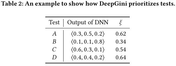
where the \mathbf{p}_ t is the probability distribution of the test t. We could easily parallelize the computation of this metric using \xi(T) = \mathbf{1} – \mathrm{diag}(\mathbf{PP}^T), where \mathbf{P} is a matrix of (n_\text{sample}, n_\text{class}). For example, to reproduce the Table 2 in the paper, we have:

import numpy as np

P = np.array([
    [0.3, 0.5, 0.2],
    [0.1, 0.1, 0.8],
    [0.6, 0.3, 0.1],
    [0.4, 0.4, 0.2]
])

xis = 1 - np.diag(np.matmul(P, P.T))
# array([0.62, 0.34, 0.54, 0.64])

image-20230827182742854

Some comments on this metric:

  • This metric is equivalent to entropy as the only different is an additional log term and a scalar.
  • This metric is exactly the same as the Gini score used in the decision trees (see sklearn doc).

Evaluation Metrics

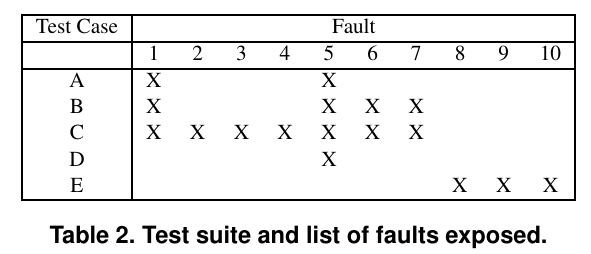
Average Percentage of Fault-Detection (APFD) was first defined in [2], which first proposes the test case prioritization problem. The example below comes from that paper.

Suppose we have a program of 10 known faults and a suite of 5 test cases; each test case is able to detect a subset of faults, then we have the following table:

A B C D E
Test Suites Used (x-axis) 1/5 2/5 3/5 4/5 1
Faults Detected (y-axis) 1/5 2/5 7/10 7/10 1

Then we could compute the APFD with the statistics provided (answer); this answer agrees with what is provided in the paper (Figure 1).

import numpy as np

xs = np.linspace(0, 1, 6)
ys = [0, 1/5, 2/5, 7/10, 7/10, 1]

apfd = np.sum(np.diff(xs) * (ys[:-1] + np.diff(ys)/2))
# 0.5

image-20230827163319793

For machine learning models, the APFD is defined differently as 1 – \frac{1}{kn} \sum_{i=1}^k o_i + \frac{1} {2n}, where k of the total n tests are misclassified, and o_i is the index of the first test that revealls i-th misclassified test.

Experiments

  • The experiments in the paper prioritize (1) the original test splits of some image classification datasets, and (2) the adversarial attacked versions of these datasets using standard approaches like FGSM.
  • There are two issues with the paper:
    • This paper does not consider the OOD test sets.
    • The paper tries to augment the training set with the attacked test examples to improve the classification accuracy. It is more sensible to augment the training sets with external annotated datasets.

Reference

  1. Regression testing minimization, selection and prioritization: a survey (published 2012; more than 1K citations).
  2. Test Case Prioritization: An Empirical Study (ICSM ’99; ICSM renamed as ICSME in 2014): This paper first proposes the test case prioritization problem and the APFD metric.

Reading Notes | Data Selection for Language Models via Importance Resampling

[Semantic Scholar] – [Code] – [Tweet] – [Video]

  • 2023-08-25: First draft. This paper is a preprint.

Problem Settings

The paper tries to solve the data selection problem for language model pretraining. Suppose a collection of high-quality samples x_ 1′ \cdots, x_ n’ have a distribution p, with another collection of N low-quality samples available; how could we sample a high-quality subset x_ 1, \cdots, x_ k\quad (k \ll N) with an underlying distribution q that approximates p?

Heuristic Classification

This is the approach used by GPT-3, EleutherAI’s Pile dataset, PaLM to select training corpus. Specifically,

  • Training a fasttext regression model f: \mathcal{X} \rightarrow [0, 1] using unigrams and bigrams from high-quality datasets.

  • Applying the trained classifier to the low-quality data collection and sampling x_ i if np.random.pareto(alpha) > 1 - score. alpha is chosen as 9 in the GPT-3 paper:

    We chose \alpha=9 in order to take mostly documents the classifier scored highly, but still include some documents that were out of distribution.

    Samples from the Pareto distributions are small; this makes most of the included samples high-quality.

Data Selection with Importance Resampling (DSIR)

The issue of the heuristic classification is that it does not explicitly model the underlying distribution q. Instead, the authors of DSIR explicitly model the distribution of a corpus as follows:

p(z; \gamma)=\prod_ {j=1}^{10000} \gamma_ j^{z_ j}

where

  • $z$ is a 10000-dimensional vector; its entries represent the index of the hashed unigrams and bigrams (with potential collisions).
  • $\gamma$ is the parameter to learn.

After learning the distributions p and q, we could assign a weight to each sample of the pool w_ i = \frac{p(z_ i)}{q(z_ i)},\ i =1, \cdots, N. We could then sample the pool with weights w_ 1, \cdots, w_ N until we have collected k samples. The authors sample the data without replacement and explain this choice theoretically. They could have explained it better, as deduplication is one key aspect for language model pretraining (Falcon paper).

Experiments

  • The average KL reduction strongly correlates (r = 0.89) with the accuracies on the downstream task (i.e., GLUE). The DSIR significantly improves the downstream accuracies. This correlation is a post-hoc justification of dataset modeling p(z;\gamma).

    The KL reduction is defined as following, where \hat{p} is target distribution, \hat{q} is the raw distribution, and p’ is the distribution of doing some data selection, including random selection, expert curation, and sampling with the proposed algorithm.

    \frac{1}{\vert \mathcal{T}\vert} \sum_{\hat{p} \sim \mathcal{T}} \mathrm{KL}(\hat{p} \parallel \hat{q}) – \mathrm{KL}(\hat{p} \parallel p’),\quad \mathrm{KL}(p\parallel q)= H(p, q) – H(p)

    There is \mathcal{T} because the authors are trying to evaluate the data selection methods; these methods could be applied to many different models. Therefore, there will be n scores for n data selection algorithms.

  • Continued pretraining on RoBERTa on domain-specific datasets sampled using the DSIR algorithm improves upon the model fine-tuned with datasets sampled with the baseline methods (Table 1, 2).

  • Training BERT from scratch using data sampled with the different sampling approaches and fine-tuning on GLUE shows the proposed selection algorithm’s advantages over the heuristic classification and random selection (Table 4).
  • It is important to make sure the domain of the pretraining dataset matches the deployment domain as (1) performance typically drops when the domain is different (Table 3), and (2) domain transfer is hard to predict (Figure 3).

Code

The implementation of the DSIR algorithm is straightforward:

  • Obtaining the Count Vector of a String

    A count vector of text could be obtained with get_ngram_info(text) (i.e., z = h(x)). The hash_buckets returns an integer of [0, 9999].

    from nltk import WordPunctTokenizer
    
    tokenizer = WordPunctTokenizer()
    def hash_buckets(string, num_buckets=10000):
      return int(abs(hash(string)) % num_buckets)
    
    def get_ngram_info(line, n=2, num_buckets=10000):
      words = tokenizer.tokenize(line.lower())
      # "i love it" be be converted to:
      # - unigrams: ['i', 'love', 'it']
      # - bigrams: [('i', 'love'), ('love', 'it')]
      unigrams, bigrams = words, list(zip(words, islice(words, 1, None)))
    
      counts = np.zeros(num_buckets, dtype=int)
      for unigram in unigrams:
          counts[hash_buckets(unigram, num_buckets=num_buckets)] += 1
      for bigram in bigrams:
          counts[hash_buckets(bigram, num_buckets=num_buckets)] += 1
      return counts
    
  • Obtaining the Importance Weight

    The code snippet reads each line from the Pile dataset and assigns a score logratio to this line. The logratio will be used for sampling.

    log_diff_dist = np.log(target_dist + 1e-8) - np.log(pile_dist + 1e-8)
    
    with open(path, 'r') as f:
      lines = f.readlines()
    
      for k, line in enumerate(tqdm(lines, miniters=1000000, maxinterval=1000000)):
          ex = json.loads(line)
          line = ex["contents"]
    
          curr_count = get_ngram_info(line, n=ngrams)
          logratio = np.inner(curr_count, log_diff_dist)
          logratios.append(logratio)
    
  • Sample Selection

    Gumbel distribution is used to model the distribution of maximum values. The authors use it here to make sure the sampling is done without replacement (i.e., Gumbel top-k trick).

    logratios = logratios
    logratios += np.random.gumbel(size=len(logratios))
    
    # select the samples with lowest logratios
    chosen_idxs = np.argpartition(-logratios, num_to_retrieve)[:num_to_retrieve]
    

Based on the functions above, we could write a simple unified function select_data_using_dsir(source_df, target_df, num_to_retrieve). This function is applicable to the scenario where both the source and target dataset are not too large and could be processed in memory.

def select_data_using_dsir(source_df, target_df, num_to_retrieve):
    source_texts = source_df.text.tolist()
    target_texts = target_df.text.tolist()

    source_count_vecs = [
        get_ngram_info(source_text) for source_text in tqdm(source_texts, desc="modeling source texts")
    ]

    source_dist = np.sum(source_count_vecs, axis=0)
    target_dist = np.sum(
        [get_ngram_info(target_text) for target_text in tqdm(target_texts, desc="modeling target texts")],
        axis=0
    )

    source_dist = source_dist / source_dist.sum()
    target_dist = target_dist / target_dist.sum()

    log_diff_dist = np.log(target_dist + 1e-8) - np.log(source_dist + 1e-8)
    logratios = np.array([
        np.inner(source_count_vec, log_diff_dist)
        for source_count_vec in tqdm(source_count_vecs, desc="retrieving source texts")
    ])
    logratios += np.random.gumbel(size=len(logratios))

    source_df["score"] = logratios
    chosen_idxs = np.argpartition(-logratios, num_to_retrieve)[:num_to_retrieve]

    return source_df.iloc[chosen_idxs]

source_dataset = load_dataset('yxchar/imdb-tlm', split="train")
target_dataset = load_dataset("yxchar/ag-tlm", split="train")

source_df = pd.DataFrame(source_dataset)
target_df = pd.DataFrame(target_dataset)

selected_source_df = select_data_using_dsir(source_df, target_df, num_to_retrieve=100)
Reading Notes | Out-of-Distribution Detection and Selective Generation for Conditional Language Models

Overview

The paper proposes to teach the encoder-decoder language models (the Transformers model on translation task and the PEGASUS model on summarization task) to abstain when receiving sentences substantial different from the training distribution; abstaining from generating some contents (more metaphorically, saying “I don’t know” when “I” really do not know) is indicates that the system is trustworthy; this practice improves the system safety.

Method

Given a domain-specific dataset \mathcal{D}_1 ={(x_1, y_1), \cdots, (x_N, y_N)} and a general-domain dataset (for example, C4) \mathcal{D}_0, the authors fit 4 Mahalanobis distance metrics using the representations of a model f(\cdot). The Mahalanobis distance is defined as \mathrm{MD}(\mathbf{x}; \mu, \Sigma) = (\mathbf{x} – \mu )^T \Sigma^{-1} (\mathbf{x} – \mu ); it is equivalent to -\log \mathcal{N}(\mu, \Sigma) up to a constant and a scalar difference.

Notation Fitting the Distance Metric On
$\mathrm{MD}_0(\cdot)$ $\mathcal{D}_0$
$\mathrm{MD}_\text{input}(\cdot)$ ${x_1, \cdots, x_N}$
$\mathrm{MD}_\text{output}(\cdot)$ ${y_1, \cdots, y_N}$
$\mathrm{MD}_\delta(\cdot)$ ${f(x_1), \cdots, f(x_N)}$

Then the authors use either of the following two metrics to compute the OOD score of a test sample z; the w is decoded output of z. The idea of using relative distance comes from authors’ previous work on selective classification (see [3]).

  • Input Relative MD (RMD) Score: \mathrm{RMD}_ \text{input}(z) = \mathrm{MD}_ \text{input}(z) – \mathrm{MD}_0(z).
  • Output Relative MD (RMD) Score: \mathrm{RMD}_ \text{ouput}(w) = \mathrm{MD}_ \text{output}(w) – \mathrm{MD}_\delta(w).

If the scores indicate that the test sample z is an anomaly, the language model abstains from generating actual w; rather, it generates preset content such as “I don’t know.”

Experiments

  • Perplexity should not be used for OOD detection alone because
    • The fitted PDFs of perplexities on different datasets (i.e., domains) mostly overlap (Figure 1).
    • When the averaged OOD scores increase, the Kentall’s \tau between perplexity and quality measure is (1) low and (2) decreases (Figure 4). If perplexity is a good measure, then the curve should be mostly flat.
    • It could be combined with the proposed metric (Section 4.3, 4.4).
  • The proposed metrics perform differently for different types of tasks: \mathrm{RMD}_ \text{input}(\cdot) is more suitable for translation task and \mathrm{RMD}_ \text{output}(\cdot) is more suitable for summarization task. This may be because the summarization task is more “open-ended” than translation task.

  • The distance between domains could be quantitatively measured with the Jaccard similarity of n-grams (1 through 4 in the paper) (Table A.10). This is used to quantify the task difficulties as the authors define “near OOD” and “far OOD” domains (Table 1).

References

  1. [1705.08500] Selective Classification for Deep Neural Networks

  2. [1612.01474] Simple and Scalable Predictive Uncertainty Estimation using Deep Ensembles: This paper works on predictive uncertainty of deep classification models. Their proposed approach tries to approximate the state-of-the-art Bayesian NNs while being easy to implement and parallelize.

  3. [2106.09022] A Simple Fix to Mahalanobis Distance for Improving Near-OOD Detection: For a classification problem of K classes, we could fit K class-dependent Gaussian and 1 background Gaussian. Then we could use these (K+1) Gaussians to detect anomalies: a negative score in class k indicates that the sample is in the domain k and a positive score means it is OOD; a more positive score shows that the sample deviates more from that domain.