[Semantic Scholar] – [Code] – [Tweet] – [Video] – [Website] – [Slide]

Change Logs:

• 2023-10-06: First draft. This paper appears at NeurIPS 2020.

Method

Given a query x, the RAG system first retrieves z from traditional index (for example, Wikipedia) based on a DPR model p _ \eta(z \vert x). Then the generator generates answers in the free text form through p _ \theta (y _i \vert x, z, y _ {1:i-1}), where y _ {1:i-1} is a prompt. In this process, the z is a latent variable that is not observable by the users.

• Note: The ability to generate answer in the free-text form is impressive because many of the experimented tasks are extractive.

The RAG system could be trained jointly on p _ \eta and p _ \theta as it is end-to-end differentiable. The authors provide two variants of the RAG system:

• RAG-Sequence: For a query, the entire output sequence is conditioned on the same document.
• RAG-Token: For a query, each token in the output sequence could be conditioned on the different documents. The authors note that the RAG could be used for knowledge-intensive tagging task:

  Finally, we note that RAG can be used for sequence classification tasks by considering the target class as a target sequence of length one, in which case RAG-Sequence and RAG-Token are equivalent.

Note that RAG-Token does not seem to much better than RAG-Sequence but the former has much more downloads on HuggingFace.

Specifically, the retrieval model is based on bert-base-uncased and the generator is based on facebook/bart-large. Importantly, to accelerate the training, document encoder is frozen and gradients only travel to the query encoder; this design choice does not hurt performance.

Additional Notes

• The benefits of RAG is that the index could be updated on demand (“hot-swapping” in the paper).

[Semantic Scholar] – [Code] – [Tweet] – [Video] – [Website] – [Slide]

Change Logs:

• 2023-10-05: First draft. This paper appears at EMNLP 2020.

Overview

• Dense Passage Retrieval is a familiar thing proposed in this paper. The issue is that previous solutions underperform BM25. The contribution of this paper is discovering an engineering feasible solution that learns a DPR model effectively without many examples; it improves upon the BM25 by a large margin.

Method

The training goal of DPR is to learn a metric where the distance between the query q and relevant documents p^+ smaller than that of irrelevant documents p^- in the high-dimensional space. That is, we want to minimize the loss below:
L(q _ i, p _ i ^ +, p _ {i1} ^ -, \cdots, p _ {in}^-) := -\log \frac{ \exp(q _ i^T p _ i^+)}{\exp(q_i^T p _ i ^ +) + \sum _ {j=1}^n \exp(q _ i ^ T p _ {ij}^-)}
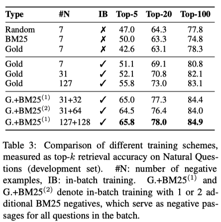
The authors find that using the “in-batch negatives” is a simple and effective negative sampling strategy (see “Gold” with and without “IB”; also see the dissection of code). Specifically, within a batch of B examples, any answer that is not associated with the current query is considered a negative. If one answer (see the bottom block) retrieved from BM25 is added as a hard negative, the performance will improve more.

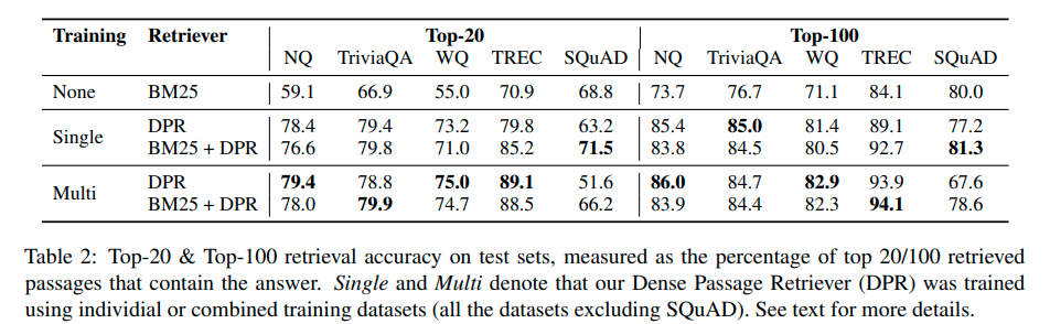
The retrieval model has been trained for 40 epochs for larger datasets (“NQ”, “TriviaQA”, “SQuAD”) and 100 epochs for smaller ones (“WQ”, “TREC”) with a learning rate 1e-5. Note that the datasets the authors use to fine-tune the models are large. For example, natural_questions is 143 GB.

Additional Notes

• The dual-encoder + cross-encoder design is a classic; they are not necessarily end-to-end differentiable. For example, in this work, after fine-tuning the dual-encoder for retrieval, the authors separately fine-tuned a QA model. This could be a favorable design due to better performance:

  This approach obtains a score of 39.8 EM, which suggests that our strategy of training a strong retriever and reader in isolation can leverage effectively available supervision, while outperforming a comparable joint training approach with a simpler design.

• The inner product of unit vectors is indeed the cosine similarity.

Quickstart

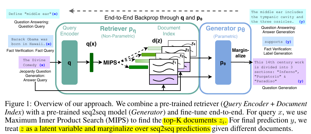
• HuggingFace provides classes for DPR. The Retrieval Augmented Generation (RAG) is one example that fine-tunes using DPR to improve knowledge-intense text generation.
• simpletransformers provides easy-to-use interfaces to train DPR models; it even provides a routine to select hard negatives. The following is a minimal working example:

import os
import logging

os.environ["WANDB_DISABLED"] = "false"
os.environ["TOKENIZERS_PARALLELISM"] = "false"

import pandas as pd
from sklearn.model_selection import train_test_split
from simpletransformers.retrieval import (
RetrievalModel,
RetrievalArgs,
)

from datasets import (
Dataset,
DatasetDict,
)

logging.basicConfig(level=logging.INFO)
transformers_logger = logging.getLogger("transformers")
transformers_logger.setLevel(logging.WARNING)

# trec_train.pkl and trec_dev.pkl are prepared from the original repository
# see: https://github.com/facebookresearch/DPR/blob/main/README.md
df = pd.read_pickle("../datasets/trec_train.pkl")
train_df, eval_df = train_test_split(df, test_size=0.2)
test_df = pd.read_pickle("../datasets/trec_dev.pkl")

columns = ["query_text", "gold_passage", "title"]

train_data = train_df[columns]
eval_data = eval_df[columns]
test_data = test_df[columns]

# Configure the model
model_args = RetrievalArgs()

model_args.num_train_epochs = 40
model_args.include_title = False

# see full list of configurations:
# https://simpletransformers.ai/docs/usage/#configuring-a-simple-transformers-model
# critical settings
model_args.learning_rate = 1e-5
model_args.num_train_epochs = 40
model_args.train_batch_size = 32
model_args.eval_batch_size = 32
model_args.gradient_accumulation_steps = 1
model_args.fp16 = False
model_args.max_seq_length = 128
model_args.n_gpu = 1
model_args.use_multiprocessing = False
model_args.use_multiprocessing_for_evaluation = False

# saving settings
model_args.no_save = False
model_args.overwrite_output_dir = True
model_args.output_dir = "outputs/"
model_args.best_model_dir = "{}/best_model".format(model_args.output_dir)
model_args.save_model_every_epoch = False
model_args.save_best_model = True
model_args.save_steps = 2000

# evaluation settings
model_args.evaluate_during_training = True
model_args.evaluate_during_training_steps = 100

# logging settings
model_args.silent = False
model_args.logging_steps = 50
model_args.wandb_project = "HateGLUE"
model_args.wandb_kwargs = {
"name": "DPR"
}

model_type = "dpr"
context_encoder_name = "facebook/dpr-ctx_encoder-single-nq-base"
question_encoder_name = "facebook/dpr-question_encoder-single-nq-base"

model = RetrievalModel(
model_type=model_type,
context_encoder_name=context_encoder_name,
query_encoder_name=question_encoder_name,
use_cuda=True,
cuda_device=0,
args=model_args
)

# Train the model
model.train_model(train_data, eval_data=eval_data)
result = model.eval_model(eval_data)

Code

This section tries to dissect the code used by simpletransformers.

• The entire process is trying to maximizing the probability of correct pairing of query and the gold passage; this is done through minimizing the negative log-softmax defined in _calculate_loss().

  Here the torch.nn.functiona.log_softmax() + torch.nn.NLLLoss() is equivalent to torch.nn.CrossEntropyLoss(); torch.nn.NLLLoss() requires the input to be the log-softmax of shape (B, C) and the label of shape (B,). For example, the output scalar of code below is -0.2.

import torch

loss = torch.nn.NLLLoss(reduction="mean")
probs = torch.diag(torch.linspace(0, 1, 5))
labels = torch.LongTensor([3, 2, 3, 4, 4])

print(loss(probs, labels))

• The effect of adding hard negatives is simply making the process of maximizing the probability of correct pairs more difficult yet conducive to the training.

class RetrievalModel:
    //...
    def _calculate_loss(
        self,
        context_model,
        query_model,
        context_inputs,
        query_inputs,
        labels,
        criterion,
    ):
        context_outputs = context_model(**context_inputs).pooler_output
        query_outputs = query_model(**query_inputs).pooler_output

        context_outputs = torch.nn.functional.dropout(context_outputs, p=0.1)
        query_outputs = torch.nn.functional.dropout(query_outputs, p=0.1)

        # (B, B) or (B, 2B) depending if there are hard negatives
        similarity_score = torch.matmul(query_outputs, context_outputs.t())
        softmax_score = torch.nn.functional.log_softmax(similarity_score, dim=-1)

        criterion = torch.nn.NLLLoss(reduction="mean")

        # for k-th row, summing up the labels[k] entry and do the average over -1/B * (l1 + l2 + ... + lB)
        loss = criterion(softmax_score, labels)

        max_score, max_idxs = torch.max(softmax_score, 1)
        correct_predictions_count = (
            (max_idxs == torch.tensor(labels)).sum().cpu().detach().numpy().item()
        )

        return loss, context_outputs, query_outputs, correct_predictions_count
    //...
    def _get_inputs_dict(self, batch, evaluate=False):
        device = self.device

        labels = [i for i in range(len(batch["context_ids"]))]
        labels = torch.tensor(labels, dtype=torch.long)

        if not evaluate:
            # Training
            labels = labels.to(device)

            # adding hard negatives will increase the number of samples
            # in each batch from B to 2B
            if self.args.hard_negatives:
                shuffled_indices = torch.randperm(len(labels))
                context_ids = torch.cat(
                    [
                        batch["context_ids"],
                        batch["hard_negative_ids"][shuffled_indices],
                    ],
                    dim=0,
                )
                context_masks = torch.cat(
                    [
                        batch["context_mask"],
                        batch["hard_negatives_mask"][shuffled_indices],
                    ],
                    dim=0,
                )
            else:
                context_ids = batch["context_ids"]
                context_masks = batch["context_mask"]
            context_input = {
                "input_ids": context_ids.to(device),
                "attention_mask": context_masks.to(device),
            }
            query_input = {
                "input_ids": batch["query_ids"].to(device),
                "attention_mask": batch["query_mask"].to(device),
            }
        else:
            # Evaluation
            shuffled_indices = torch.randperm(len(labels))

            labels = labels[shuffled_indices].to(device)

            if self.args.hard_negatives:
                context_ids = torch.cat(
                    [
                        batch["context_ids"][shuffled_indices],
                        batch["hard_negative_ids"],
                    ],
                    dim=0,
                )
                context_masks = torch.cat(
                    [
                        batch["context_mask"][shuffled_indices],
                        batch["hard_negatives_mask"],
                    ],
                    dim=0,
                )
            else:
                context_ids = batch["context_ids"][shuffled_indices]
                context_masks = batch["context_mask"][shuffled_indices]

            context_input = {
                "input_ids": context_ids.to(device),
                "attention_mask": context_masks.to(device),
            }
            query_input = {
                "input_ids": batch["query_ids"].to(device),
                "attention_mask": batch["query_mask"].to(device),
            }

        return context_input, query_input, labels