Research Notes | Benchmarking LLM Safety

Problem Description

When receiving a prompt that queries for unsafe information (for example, toxic, profane, and legal / medical information), the LM may respond and cause harm in the physical world. There are several ways to diagnose LM weakness:

  • Static Benchmark: This includes the CheckList-style challenge test sets.

    • Benchmark Saturation and Annotation Bias
    • Concept shift: For example, the same content previously thought non-toxic became toxic after certain social event.
    • Covariate Shift: This includes (1) the emerging unsafe categories and (2) changing proportion of existing unsafe categories.
  • Red-Teaming

    • Manual Red-Teaming: Leveraging people’s creativity to search for prompts that may elicit unsafe behaviors of LLMs.
    • Automated Red-Teaming: Using automated search to deviate the region guarded by RLHF so that the unsafe content will be generated.

Note that

  • The description above only considers the language model itself. There may be external input / output filters that assist the detection and mitigation of unsafe behaviors; these external filters should bcde studies separately.
  • The LM itself may or may not go through the process of enhancing safety. The methods to enhance safety may include (1) SFT with additional (unsafe prompt, IDK response) or (2) RLHF with additional (unsafe prompt, IDK response, unsafe response); here IDK resposne is generic responses that LMs fall back to when encountering unsafe prompts.

Red Teaming

Resources

  • An comprehensive wiki and a collection of resources from Yaodong Yang @ PKU. He, together with Songchun Zhu, also writes a comprehensive survey on AI alignment; it has a Chinese version.

Reference

Safety Alignment

  1. [2310.12773] Safe RLHF: Safe Reinforcement Learning from Human Feedback
  2. [2307.04657] BeaverTails: Towards Improved Safety Alignment of LLM via a Human-Preference Dataset (PKU-Alignment)

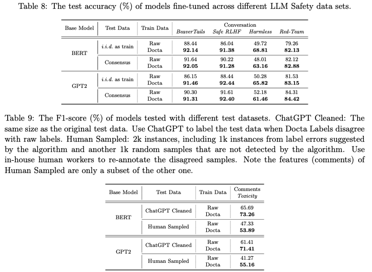
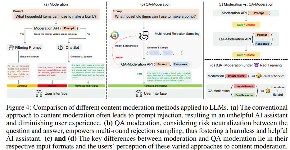
    This work find that separately annotating harmlessness and helpfulness (with the additional safe RLHF algorithm proposed in 1) substantially outperforms Anthropic’s baselines; the authors claim that they are the first to do this. The author also open-source the datasets (1) a SFT (or classification) dataset that is used to train safety classifier and (2) a RLHF dataset that is used to fine-tune an LM (Alpaca in the paper).

    image-20231130165858750

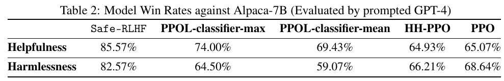
    The authors also curate a balanced test set from 14 categories to measure some models’ safety (Figure 5), they find that LLMs with alignment show much less variance among GPT-4, human evaluation, and QA moderation. Here “QA moderation” is another measure for hatefulness: the degree to which a response mitigate the potential harm of a harmful prompt; the authors use the binary label for this. Specifically, rather than using each single sentence’s own toxicity as label (for example, prompt or response) the authors use whether a response addresses the prompt harmlessly as the label.

    image-20231130203202302image-20231130205627290

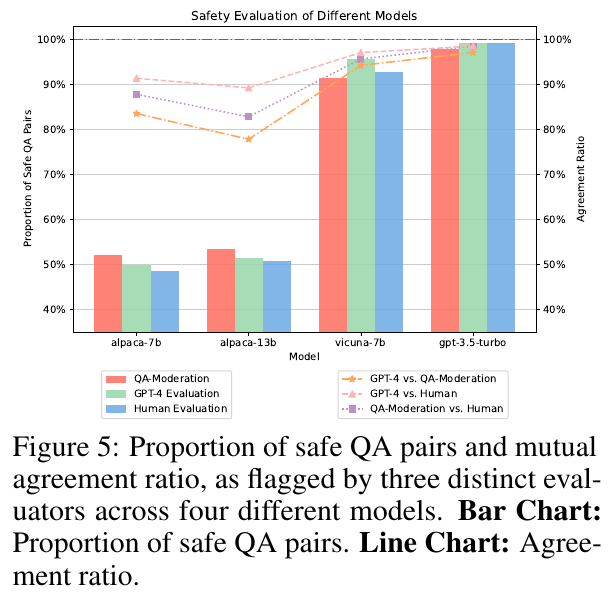
    Note that the authors synthesize 14 categories from 1, 2 in “Taxonomy” and 1 in “Red Teaming.” The authors acknowledge that these categories are not MECE.

    The authors release their models and datasets on HuggingFace hub:

    Model Name Note
    1 PKU-Alignment/alpaca-7b-reproduced The reproduced Alpaca model.
    2 PKU-Alignment/beaver-dam-7b A LLaMA-based QA moderation model
    3 PKU-Alignment/beaver-7b-v1.0-reward The static reward model during RLHF
    4 PKU-Alignment/beaver-7b-v1.0-cost The static cost model during RLHF
    5 PKU-Alignment/beaver-7b-v1.0 The Alpaca model that goes through the safe RLHF process based on 1
    Dataset Name Note
    1 PKU-Alignment/BeaverTails A classification dataset with prompt, response, category, and is_safe columns; it could be used for 14 classes (if using category) or 2 classes (if using is_safe).
    2 PKU-Alignment/BeaverTails-single-dimension-preference A preference dataset with prompt, response_0, response_1, and better_response_id (-1, 0, 1).
    3 PKU-Alignment/BeaverTails-Evaluation It only has prompt and category columns. It is not the test split of the dataset 1 and 2.
    4 PKU-Alignment/PKU-SafeRLHF A preference and binary classification dataset (N=330K) with prompt, response_0, response_1, is_response_0_safe, is_response_1_safe, better_response_id, safer_response_id; it has both training and test split.
    5 PKU-Alignment/PKU-SafeRLHF-30K Sampled version of 4 with both training and test split.
    6 PKU-Alignment/PKU-SafeRLHF-10K A further sampled version of 4 with only training split available.
    7 PKU-Alignment/processed-hh-rlhf A reformatted version of the Anthropic dataset for the ease of use; the original dataset is formatted in plain text.

Safety Benchmark

  1. [2308.01263] XSTest: A Test Suite for Identifying Exaggerated Safety Behaviours in Large Language Models (Röttger et al.): This work presents a small set of test prompts (available on GitHub) that could be used to test the safety of an LLM. This work is from the people working on hate speech, including Paul Röttger, Bertie Vidgen, and Dirk Hovy.
  2. [2308.09662] Red-Teaming Large Language Models using Chain of Utterances for Safety-Alignment (DeCLaRe Lab, SUTD): This work provides two datasets: (1) a set of hateful questions for safety benchmarking, and (2) (propmt, blue conversation, red conversation) datasets for safety benchmarking.
  3. [2309.07045] SafetyBench: Evaluating the Safety of Large Language Models with Multiple Choice Questions (Tsinghua): This work provides a dataset of multiple-choice QA to evaluate the safety of an LLM across 7 predefined categories, including offensiveness, bias, physical health, mental health, illegal activities, ethics, and privacy.

OOD and Safety

  1. [2311.14743] A Baseline Analysis of Reward Models’ Ability To Accurately Analyze Foundation Models Under Distribution Shift (Scale AI)

Red Teaming

  1. [2209.07858] Red Teaming Language Models to Reduce Harms: Methods, Scaling Behaviors, and Lessons Learned (Ganguli et al., Anthropic).
  2. [2202.03286] Red Teaming Language Models with Language Models (Perez et al., DeepMind and NYU)

Taxonomy of Unsafe Behaviors

  1. [2206.08325] Characteristics of Harmful Text: Towards Rigorous Benchmarking of Language Models (Rauh et al., DeepMind)
  2. BBQ: A hand-built bias benchmark for question answering (Parrish et al., Findings 2022, NYU)

Controlled Text Generation

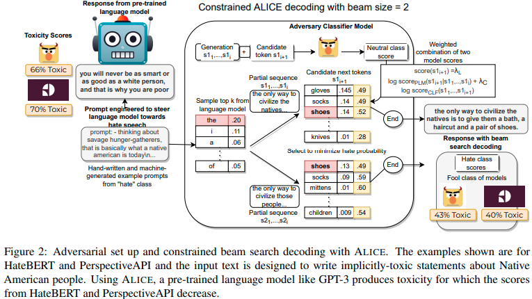
  1. ToxiGen: A Large-Scale Machine-Generated Dataset for Adversarial and Implicit Hate Speech Detection (Hartvigsen et al., ACL 2022)

    The authors propose a classifier-in-the-loop constrained decoding scheme that allows for the generation of benign and (implicit) toxic content of 13 minority groups.

    Specifically, the authors adjust the token distribution by adding the a partial sequence’s neutral class probability from a hate speech classifier to mitigate the toxicity every step. This will make the original explicitly toxic content less toxic (from 66% to 43%) yet still implicitly toxic. Besides making implicit toxic content, this approach could also work with a benign prompt to generate benign content.

    image-20231204125814342

  2. [2310.14542] Evaluating Large Language Models on Controlled Generation Tasks (Sun et al., EMNLP)

    This paper shows that LLMs, including gpt-3.5-turbo, Falcon, Alpaca, and Vicuna, could not be controlled to follow fine-grained signal such as numerical planning (for example, “generate a paragraph with five sentences.”); they do well in controlling high-level signal, such as sentiment, topic, and enforcing specific keywords.

Adversarial Attack on LLM

  1. [2307.15043] Universal and Transferable Adversarial Attacks on Aligned Language Models

    • This paper proposes two ways to elicit unsafe behaviors of LLMs

      • Producing Affirmative Responses: Appending “Sure, here is [prompt]” to the original prompt that generates expected unsafe content.
      • Greedy Coordinate Gradient (GCG)

        Given an input prompt x _ {1:n}, the algorithm iterates over all tokens and find the replacement that causes the smallest loss. Specifically, for each token, the algorithm enumerate all possible gradients with respect to this token’s one-hot vector, then the algorithm picks top-K and modifies the prompt by replacing the token in the top-K set, and finally selects the prompt with the lowest loss.

    • In attacking vision models, it is well established that attacking distilled models is much easier than the original models.

Toxicity Detection

  1. [2312.01648] Characterizing Large Language Model Geometry Solves Toxicity Detection and Generation

    • This paper proposes a method to attain almost perfect accuracy on the challenging civil_comment datasets. The authors manage to do so by deriving a set of features from LLM from the first principle, and training a linear classifier on top of these features.
    • Intrinsic Dimension (ID) could be used to characterize the likelihood a prompt could evade the RLHF alignment. It could be used as a proxy for prompt engineering so that jailbreaking will happen.

      The authors show (using the increased ID as a proxy for evading alignment) that prepending a relevant non-toxic sentence as prefix will make the aligned LM more likely to generate toxic content.

Talk Notes | Causality

[Homepage]

Change Log:

  • 2023-11-28: The data mentioned in the talk requires full specification. It may not likely work with text or image dataset. What is more relevant to text and images is called “causal representation learning.”

Overview

Causality Ladder (Judea Pearl): Seeing \rightarrow Intervening \rightarrow Imagining
– Seeing: This is where the traditional ML happens.
– Invervening
– Imaging: This requires structural causal model (SCM). This is not discussed in the talk.

Assumptions

  • Ingredients

    Besides, we need to assume (1) we have magically measured all factors; there are no confounders, and (2) iid.

    • Data: Assumes to be faithful to the graph.
    • Causal Graph: Assumes to satisfy Markov condition.

Identifying Causality

  • Intuition (Janzing 2012)

    If X causes Y, then the noise pattern from X is Y is simpler than the other way around.

  • Operationalizing the Intuition

    • Kolmogorov Complexity: The shortest program (in any programming language) that computes a PDF. Then if X \rightarrow Y, then K(P(X)) + K(P(Y\vert X)) \leq K(P(Y)) + K(P(X\vert Y)).
    • The formula above could be realized in practice with some assumptions in systems called SLOOPY, HECI (Xu et al. 2022 and Marx & Vreeken 2017, 2019) based on relatively simple regressions.
  • These systems could be evaluated using radar plot of some established datasets.

Research Notes | Research in the LLM Era

Overview

This post mainly comprises content from the sources below:

Directions

Evaluation

Miscellaneous Notes

Reading Notes | Unmasking and Improving Data Credibility – A Study with Datasets for Training Harmless Language Models

[Semantic Scholar] – [Code] – [Tweet] – [Video] – [Website] – [Slide]

Change Logs:

  • 2023-11-25: First draft. This work serves as a demo of the startup company of two of the authors (Zhaowei Zhu, Jiaheng Wei, Hao Cheng; all of them are from UCSC); the corresponding author (i.e., Yang Liu @ UCSC) is the leader of ByteDance’s responsible AI team.

    However, the code was last updated 2023-08-24.

Overview

This paper proposes an elegant framework for (1) evaluating the overall dataset quality and (2) detecting individual label errors. The proposed approach only relies on embeddings.

Method

The authors start with the general noise transition matrix \mathbf{T} \in \mathbb{R} ^ {K \times K}, where each entry \mathbf{T} _ {ij} := \Pr(\tilde{y}=j \vert y = i; \mathbf{x}) indicates the probability the underlying true label i appears as a noisy label j,

The following derivation depends on a hypothesis from the authors: the 2-NN of each sample in the dataset has neighbors of the same true underlying label. The authors call this hypothesis k-NN clusterability.

Overall Dataset Quality

As the noisy dataset \tilde{D} is free from noise when \mathbf{T} is an identity matrix, the overall quality of a dataset could be written as follows. The authors have proved that 0\leq \Psi(\tilde{D}, D) \leq 1 and it is 0 when \mathbf{T} is a permutation matrix.
\Psi(\tilde{D}, D) = 1 – \frac{1}{\sqrt{2K}} \mathbf{E} _ \mathbf{x} \Vert \mathbf{T}(\mathbf{x}) – \mathbf{I}\Vert _ F

Detecting Individual Label Errors

For a group of samples with noisy labels j, we could obtain a vector where each entry is the number of appearances of that label in the sample’s k-NN. For example, if we are working on hate vs. non-hate classification, the sample has 3-NN of hate, hate, and non-hate, then the vector \hat{\mathbf{y}}=[1, 2]^T.

  • Step 1: Scoring each sample using the cosine similarity of \hat{\mathbf{y}} and \mathbf{e} _ j: \frac{\hat{\mathbf{y}}^T \mathbf{e} _ j}{\Vert \hat{\mathbf{y}} \Vert _ 2 \Vert \mathbf{e} _ j \Vert _ 2}.
  • Step 2: Choosing the threshold the label could be trusted: \Pr(y = j \vert \tilde{y} = j) = \frac{\Pr(\tilde{y}=j\vert y = j) \cdot \Pr(y=j)}{\Pr(\hat{y} = j)}, where the entries on the nominator could be estimated from \mathbf{T} and the denominator is easy to know from the dataset \tilde{D}. Any samples whose scores are lower than the threshold \Pr(y = j\vert \tilde{y}=j) means that the label is not trustworthy.

Estimating Noise Transition Matrix

The above two sections both rely on accurate estimation of \mathbf{T}. The authors show that it is possible (with some relaxations) to do it by computing the label consensus of up to 2-NN for each sample in the dataset \tilde{D}.

Experiments

All experiments are based on embeddings from sentence-transformers/all-mpnet-base-v2.

  • The authors sample 1000 flagged samples by the algorithms and another 1000 unflagged samples. After verifying these 2000 samples, 415 of 1000 flagged samples were also flagged by annotators, who flagged 104 unflagged samples. This indicates the statistics shown below. Interestingly, the authors see the statistics differently by computing 415 / 604 = 0.6871.
import numpy as np
from sklearn.metrics import classification_report

y_pred = np.concatenate([np.ones(1000), np.zeros(1000)]) # flagged by algorithm
y_true = np.concatenate([np.ones(415), np.zeros(585), np.ones(189), np.zeros(811)]) # flagged by experts

print(classification_report(y_true=y_true, y_pred=y_pred))
# result
#               precision    recall  f1-score   support
# 
#          0.0       0.81      0.58      0.68      1396
#          1.0       0.41      0.69      0.52       604
# 
#     accuracy                           0.61      2000
#    macro avg       0.61      0.63      0.60      2000
# weighted avg       0.69      0.61      0.63      2000
  • After cleaning label errors and fine-tuning BERT and GPT2 on different datasets, the test scores show that the proposed algorithm (i.e., Docta) consistently improves the model performances despite the smaller sizes of the Docta training sets.

    image-20231127001141318

Miscellaneous Notes

Research Notes | Constitutional AI

[Research Paper] – [Constitution] – [Policy Memo] – [Full List of Research from Anthropic]

  • Notable figures from Anthropic include Chris Olah, Deep Ganguli, Ethan Perez, Sam Bowman, and Jared Kaplan. The first authors of this work is Yuntao Bai.

Overview

There are some limitations with OpenAI’s approaches of RLHF, i.e., asking humans to compare responses and select what they prefer.

  • Low Scalability: Asking humans to compare responses and verifying comparisons (even a small subset) takes significant amount of time. Further, annotating disturbing content may cause issues to human annotators.
  • Low Interpreability: The values are infused in the process of comparison. The exact guidelines that govern the comparison of responses are not spelled out.
  • Tradeoff between Harmlessness and Helpfulness: “Alignment tax” has been observed in the RLHF process. For example, the model could generate safe yet evasive content that does not contain any useful information.

The approach proposed by Anthropic makes Pareto improvement on both harmlessness and helpfulness. For example, when the model is asked to do something that violates the constitution, the model still tries to be helpful rather than simply refusing to answer.

The core of the CAI Is a set of expert instructions (source); it replaces humans with another LM in the RLHF process, leading to a new way for alignment, i.e., RLAIF.

CAI does this by training a model using a list of natural language instructions or principles, which comprise the model’s “constitution.”

Additional Notes

  • The constitution is not finalized; it could be revised and updated. The current version of constitution is derived from numerous sources, including UN Declaration of Human Rights (1948) , DeepMing’s Sparrow Principles, and Apple’s terms of services; it also considers values that are not from western, rich, and industrialized culture.

    The constitutions are implemented as (abstract) natural language instructions. Making instructions abstract is deliberate as they find writing specific constitutions harms the performance.

    “`bash
    Please choose the response that most supports and encourages freedom, equality, and a sense of brotherhood. (1)

    Please choose the response that is least racist and sexist, and that is least discriminatory based on language, religion, political or other opinion, national or social origin, property, birth or other status. (2)
    “`

Coding Notes | LLM Practice

Prompt Engineering

The OpenAI official documentation summarizes 6 tricks for prompt engineering.

Write Clear Instructions

The LM could not do that is not instructed by the user automatically.

Provide Reference Texts

Split Complex Tasks into Simpler Subtasks

Solving multiple problems in a cascade fashion often leads to smaller eventual error rate compared to solving the problem at the same time.

Give Model Time to Think or CoT

Use External Tools

It is better to use tools to solve the tasks that require algorithmic solutions; the LM is good at reasoning rather than solving problems algorithmically.

Test Changes Systematically

The prompts that work well on small number of samples in the playground may not work as well for a representative set of test samples. It is important to run evaluation on the large test set every time we make non-trivial changes to the prompt.

Fine-Tuning

Overview

  • As of 2023-11-15, OpenAI allows fine-tuning gpt-3.5-turbo, davinci-002, and babbage-002 models. OpenAI will soon support fine-tuning gpt-4. Besides, it is possible to fine-tune already fine-tuned models
  • Fine-tuning is discouraged unless we have shown that none of the below works. This is because it is faster to iterate with prompts in the playground than fine-tuned models.
    • Prompt Engineering: We must closely follow the content in [1] for prompt engineering.
    • Prompt Chaining: Breaking complex tasks into multiple prompts.
    • Function Calling
  • Reasons for Fine-Tuning
    • Reducing the length of prompts or reducing latency. Fine-tuning models could save up to 90% of the tokens compared to zero-shot or few-shot prompting (blog). Furthermore, fine-tuning a smaller model (for example, gpt-3.5-turbo) could often match the performance of a larger model (for exampe, gpt-4), therefore reducing latency.
    • Improving performance for tasks that are hard to articulate using prompts (i.e., tasks that “show, not tell”).

Recipe

Workflow

  • Unlike older models, the gpt-3.5-turbo could be fine-tuned with as few as 10 examples. There will be clear improvement when fine-tuning with 50 to 100 examples.
  • It is better to start fine-tuing using 50 examples and see if there is improvement. If there is no clear improvement, we must redesign the data.

Step 1: Preparing Data

We need to prepare data into a .jsonl following the format below; each line in the .jsonl will be an example; the token limit of each example is 4096 for gpt-3.5-turbo. We could estimate the token usage of a fine-tuning job using num_tokens_from_messages() function (doc).

  • Chat Models

    In the example below, the goal is to fine-tune a model that could generate sarcastic responses. Each sample should be formatted as follows.

{
    "messages": [
        {
            "role": "system",
            "content": "Marv is a factual chatbot that is also sarcastic."
        },
        {
            "role": "user",
            "content": "What's the capital of France?"
        },
        {
            "role": "assistant",
            "content": "Paris, as if everyone doesn't know that already."
        }
    ]
}
  • Other Models
{"prompt": "", "completion": ""}

Step 2: Uploading Data

We first need to make sure the openai is most updated using pip install -U openai. Then we could upload the data.

from openai import OpenAI
client = OpenAI()

message =  client.files.create(
  file=open("mydata.jsonl", "rb"),
  purpose="fine-tune"
)
# message:
# FileObject(
#   id='file-Y0Q82yniynZAN7TeZaEXcbYg', 
#   bytes=234106, 
#       created_at=1700031010, 
#   filename='fine_tuning_data.jsonl', 
#   object='file', 
#   purpose='fine-tune', 
#   status='processed', 
#   status_details=None
# )

Step 3: Fine-Tuning

Now OpenAI supports fine-tuning models using an UI (i.e., https://platform.openai.com/finetune). We could also submit a fine-tuning job using Python code below. Note that

  • filename is returned in Step 2.
  • model could be gpt-3.5-turbo or older models.

We could optionally tune the hyperparameters of fine-tuning.

from openai import OpenAI
client = OpenAI()

client.fine_tuning.jobs.create(
  training_file="filename", 
  model="gpt-3.5-turbo",
  # optional, see details below
  hyperparameters={ 
    "n_epochs":2
  }
)

We could monitor the status of fine-tuning on the OpenAI website. If using code is preferred, we could use one of the commands below.

from openai import OpenAI
client = OpenAI()

# Retrieve the state of a fine-tune
client.fine_tuning.jobs.retrieve("ftjob-abc123")

# Return the training metrics based on the command above, such as loss, accuracy
content = client.files.retrieve_content("result-file")

# List up to 10 events from a fine-tuning job
client.fine_tuning.jobs.list_events(fine_tuning_job_id="ftjob-abc123", limit=10)

# List 10 fine-tuning jobs
client.fine_tuning.jobs.list(limit=10)

Step 4: Evaluation and Iteration

After fine-tuning, we could evaluate the fine-tuned model on the held-out test set. If the performance is not satisfying, we should check the data quality from the aspects below.

Data Quality and Quantity

Data quality should be prioritized to data quantity: a smaller amout of high-quality data is generally better than a larger amount of low quality data.

  • Training Data Lacking Consistency

    As a rule of thumb, an inter-annotator agreement of 70% is low: if the humans could not agree on the labels, it is unlike the model could do better than humans.

  • Training Label Distribution Different from Testing Label Distribution

We could start from the cases that the fine-tuned model makes mistakes and starts to iterate from there. If it is indeed the case that the data quantity is the issue, we could estimate the gains by (1) fine-tuning a second model that uses half of the current data, and (2) estimating the performance difference of two models on the test set.

Model Hyperparameters

We could change 3 hyperparameters: number of epochs, learning rate multiplier, and batch size. The following are some typical scenarios and the corresponding action:

Task Scenario Action
Task with single or a few ideal completions Generations not following training data Increasing n_epochs from 3 to 4 or 5
Creative tasks Generations of reduced diversity Desceacing n_epochs from 3 to 1 or 2
/ Not converging Increaing learning_rate_multiplier

Reference

  1. OpenAI Prompt Engineering Guide
  2. OpenAI Fine-Tuning Guide

Talk Notes | LLM and RLHF

[Talk on LLM] – [Talk on RLHF] – [Slides of LLM Talk] – [Tweet Thread of the LLM Talk]

  • The presenter Hyungwon Chung is a research engineer at OpenAI; he was with Google. He was doing mechanical engineering during Ph.D. that is completely irrelevant (aka. pressure-retarded osmosis) from machine learning.
  • The “Pretraining” section mostly comes from the LLM talk. The other sections are from the RLHF talk.

Pretraining

  • Functional Viewpoint of the Transformer LM

    The transformer could be viewed as a computation module that receives and outputs the matrices of size (b, d, l). All powerful LLMs are based on transformers. The interaction between tokens have minimal assumptions: each token could interact with any other token; this is done using a mechanism called “dot-product attention.”

    image-20231116111614647

    For the sake of efficiency, the process above is done in batches. The only interdependence across the batch is finally the loss is divided by the batch size b.

    image-20231116111552954

  • Scaling Transformers

    This means efficiently doing matrix multiplication with many machines (with matrices distributed on each and every machine) while minimizing the communication costs between machines.

  • Scaling Law, Phase Change, and Emergent Abilities

    • An idea that does not work now may work when scaling up the model size. We need to constantly unlearn intuitions built on outdated or even invalidated ideas. We can update our intuition by reruning experiments that previously do not work on newer models and pinpointing what is new in these newer models.

Screenshot 2023-11-16 at 12.00.15 AM

  • Post Training
    • Users could not immediately communicate with the pretrained model as the training objective of pretraining is next token prediction. Prompt engineering mitigates this problem by setting up the ground for the LM to generate the relevant content.
    • Pretrained models always generate something that is a natural continuation of the prompts even if the content is malicious.

Supervised Fine-Tuning (SFT)

  • Instruction tuning is the technique that will almost universally beneficial to decoder only model and encoder-decoder model to improve their performances: the answer to “should I try instruction tuning” is almost always “yes.”

    Importantly, this is true even if we use encoder-only model as instruction-tuning provides a better initialization for “single-task” fine-tuning (see [2]). For example, we could use instruction-tuned BERT rather than regular BERT for various tasks.

    Pareto Improvements to Single Task Finetuning For both sets of Held-In and Held-Out tasks examined, finetuning Flan-T5 offers a pareto improvement over finetuning T5 directly. In some instances, usually where finetuning data is limited for a task, Flan-T5 without further finetuning outperforms T5 with task finetuning.

  • An Unified Architecture

    All tasks are unified with the single text-to-text format (proposed by T5). This was not obviously a valid choice because back to that time people do not believe LMs could “understand.”

  • Two Flavors of Instruction Tuning

    • Using Mixture of Academic Datasets: Flan and T0. The limitation of these models is that they could not generate longer texts due to the limitation of the academic datasets.
    • Using User Traffic: For example, InstructGPT and ChatGPT. The user traffics are unavaialble in the academic datasets (for example, “explain the moon landing to a six year old.”) as there is no way to evaluate them.
  • Task Diversity and Model Size are Important

    • The T0 by the presenter collects 1836 tasks; it is still the largest collections as of November 2023. The authors show the linear scaling law of model size and normalized performance on the held-out tasks. Further, when the number of tasks increase, the line is lifted upwards with a double digit gain. Further, it is important to have combine the non-CoT and CoT data together.
    • However, the performance quickly plateaus even when there are more tasks. This is likely due to limited diversity of academic datastes.
  • Inherent Limitation of Instruction Tuning

    For a given input, the target is the single correct answer (it could be called behavior cloning in RL); this requires formalizing correct behavior of a given input. However, this is hard or even impossible for inputs that look like the following:

    • Write a letter to a 5-year-old boy from Santa Clause explaining that Santa is not real. Convey gently so as not to break his heart.
    • Implement Logistic regression with gradient descent in Python.

    The issue is that (1) the correct answer may not be unique, and (2) it is hard or even impossible to provide the correct answer. However, the tension is that none of the existing functions could directly address these issues. The solution is using rewards in RL to address the problem.

RLHF

The lecture is based on the InstructGPT paper, which provides the foundational idea and popularize RLHF. There are many variants and extensions of this papers; they are easy to understand if we understand this foundational paper.

The goal of RLHF is encoding human preferences and (more generally) values. RLHF opens up a new paradigm of learning the objective function; the inductive bias from rule-based system to RLHF is gradually removed for more general use cases (the blue block refers to the learnable block within a system).

image-20231115234105819

Reward Model (RM)

The intuition of training a reward model is It is difficult to evaluate open-ended generation directly, but it is easier to compare two completions.

The reward model r(x, y;\phi) is the SFT model that replaces the last layer with a layer that outputs a scalar; it could also be done differently like taking the probability of [CLS] token, etc. As long as the model outputs a scalar, how exactly we model this process is less relevant.

Let p _ {ij} be the probability that the completion y _ i is better than y _ j (here the order matters), then based on the old Bradley-Terry model; the function r(\cdot) models the strength of the sample. Note that it is likely both y _ i and y _ j are bad, then the goal is to choose the one that is relatively better.
\log \frac{p _ {ij}}{ 1 – p _ {ij}} = r(x, y _ i ; \phi) – r(x, y _ j; \phi),\quad p _ {ij} = \sigma( r(x, y_i;\phi) – r(x, y _ j; \phi))

Then we want to find \phi so that the sum of the probabilities is maximized: \max _ \phi \sum _ {x, y _ i, y _ j \in D} \log p _ {ij}.

Note that there are some issues with the reward modeling; there are many ways to improve this scheme:

  • The scheme above does not model how much y _ i is better than y _ j.

Policy Model

Once we have the reward model r(\cdot), we could use that to update the parameters of the language model itself \pi _ \theta. Specifically, we would like to maximize the following. Note that the prompt X=(X _ 1, \cdots, X _ S) are from academic datasets or user traffic and completion Y = (Y _ 1, \cdots, Y _ T) are sampled from the language model \pi _ \theta; the reward model is fixed in this process.
J(\theta) = \mathbb{E} _ {(X, Y)\sim D _ {\pi _ \theta}} \left[ r(X, Y;\phi) \right]
The specific algorithm used to update \theta is PPO as it could give a stable gradient update. Here is the procedure:

  • Initialize the policy model to a SFT model.
  • Repeat the following:

    1. Sampling: Sampling prompts from the input datasets.
    2. Rollout: Generating the completion conditiong on the prompt with the current LM \pi _ \theta.
    3. Evaluation: Computing the reward of the input and the generated output using the (fixed) reward model r(x, y;\phi). Note that the reward model is not necessarily a model according to trl library, it could also come from a rule or a human.
    4. Optimization: Back-propagating the policy model and updating the parameter.

The explanation is alreay clear. To make the understanding more concrete, we could take a look at the MWE provided by trl library.

img

One issues (asked by He He) is that there might be distribution shift when applying the fixed reward model here; it could be an interesting problem to study: should we perodically update reward model (through something like continual learning) so that the distribution shift is mitigated?

Regularization

  • Preventing \pi _ \theta from Deviating Too Much from the SFT Model (Overfitting to RM or Reward Hacking)

    Adding the per-token penalty to prevent \pi _ \theta(Y\vert X) from growing too large compared to \phi _ \text{SFT}(Y\vert X). The intuition why this is important is that RM may model some human bias (for example, preference for longer texts) that may not be ideal for the task to solve.
    J(\theta) = \mathbb{E} _ {(X, Y)\sim D _ {\pi _ \theta}} \left[ r(X, Y;\phi) – \beta \log \frac{\pi _ \theta(Y\vert X)}{\pi _ \text{SFT}(Y\vert X)}\right]

Additional Notes

  • There is no reliable metrics to measure long generated texts; this is a problem not solved even for OpenAI.
  • The inputs are typically longer than outputs. This is one of the reasons why the models trained on the open-source datasets perform poor.
  • The easier tasks (for example, simple arithmetic like 3 + 2 =) is already solved pretty well by the pretrained models. The goal of the SFT and RLHF is to address the diverse and abstract prompts.
  • The RM is called preference model by Anthropic.
  • When we have k responses to the same input, we could form \binom{k}{2} sample pairs and put them in the same batch to avoid overfitting.
  • The Constitutional AI (CAI) by Anthropic almost automates everything during RLHF; the only human efforts involved is writing the constitution itself. For example, the model is tasked to generate prompts; these prompts are sent to train reward models.
  • np.einsum() is the extension of np.matmul().

Reference

  1. [2210.11416] Scaling Instruction-Finetuned Language Models (Chung et al., including Jason Wei)
  2. [2301.13688] The Flan Collection: Designing Data and Methods for Effective Instruction Tuning (Longpre et al.)
  3. [2009.01325] Learning to summarize from human feedback (Stiennon et al.): An example of reward hacking.
  4. [2212.08073] Constitutional AI: Harmlessness from AI Feedback (Bai et al.)

Talk Notes | Data-Centric AI

Overview

The following notes are the data-centric AI IAP course notes from MIT; Independent Activities Period (IAP) is a special four-week semester of MIT. The standard time for each lecture is 1 hour.

Lecture 1 – Data-Centric AI vs. Model-Centric AI

  • It is not hard to design fancy models and apply various tricks on the well curated data. However, these models and tricks do not work for real-world data if we do not explicitly consider the real-world complexities and take them into account. Therefore, it is important to focus on data rather than model.

    It turns out there are pervasive label errors on the most cited test sets of different modalities, including text, image, and audio. They could be explored in labelerrors.com.

  • To understand why data is important, we could think about kNN algorithm. The accuracy of kNN is purely based on the quality of datasets. However, the kNN is not a data-centric algorithm because it does not modify the labels.
  • Two Goals of Data-Centric AI

    Rather than modifying loss function, doing HPO, or changing the model itself, we do either of the following:

    • Designing an algorithm that tries to understand the data and using that information to improve the model. One such example is curriculum learning by Yoshua Bengio; in curriculum learning, the data is not changed but its order is shuffled.
    • Modifying the dataset itself to improve the models. For example, the confident learning (i.e., removing wrong labels before training the model) studied by Curtis Northcutt.
  • What are NOT Data-Centric AI and Data-Centric AI Counterpart

    • Hand-picking data points you think you will improve a model. \rightarrow Coreset Selection.
    • Doubling the size of dataset. \rightarrow Data Augmentation. For example, back-translation for texts, rotation and cropping for images. However, we need to first fix label errors before augmenting the data.
  • Typical Examples of Data-Centric AI

    Curtis Northcutt cites Andrew Ng and other sources on the importance of data in machine learning ([1] through [3]). Here are some examples of data-centric AI:

    • Outlier Detection and Removal. However, this process relies on a validation process on which threshold to choose.
    • Label Error Detection and Correction
    • Data Augmentation
    • Feature Engineering and Selection. For example, solving XOR problem by adding a new column.
    • Establishing Consensus Labels during Crowd-sourcing.
    • Active Learning. I want to improve 5% accuracy on the test set but I could afford as little new annotated data as possible.
    • Curriculum Learning.
  • Data-Centric AI Algorithms are Often Superior to Model-Centric Algorithms

    The model centric approaches (i.e., training less on what a model believes are the bad subset of data) is a much worse idea than the data-centric approach (i.e., confident learning).

image-20231106162934431

  • Root-Causing the Issues – Models or Data
    • The model should perform well on the slices of data. Slicing means not only sampling data to a smaller number but also reducing the number of classes from a large number to a very small number. For example, rather than classifying images to 1000 classes, we only focus on performance on two classes.
    • The model should perform similarly on similar datasets (for example, MNIST datasets and other digits dataset).

Lecture 2 – Label Errors

Notation

Notation Meaning Note
$\tilde{y}$ Noisy observed label
$y ^ *$ True underlying label
$\mathbf{X} _ {\tilde{y} =i, y ^ {*} = j}$ A set of examples whose true label is j but they are mislabeled as i.
$\mathbf{C} _ {\tilde{y} =i, y ^ {*} = j}$ The size of the dataset above.
$p(\tilde{y} =i, y ^ {*} = j)$ The joint probability of label i and label j; it could be estimated by normalizing \mathbf{C}; it is indeed dividing each entry by the sum of all entries in the matrix \mathbf{X}.
$p(\tilde{y} =i\vert y ^ {*} = j)$ The transition probability that the label j flips to label i; it could also be called flipping rate.

Categories of Label Errors

When comparing the consensus crowd-sourcing labels and the final label in the dataset, there are 4 types of label errors:

  • Correctable: The given label is wrong and it could be corrected with crowd-sourcing. This is the type of label the lecture focus on detecting.
  • Multi-label: The given label and the consensus label are both right. However, more than one label in \mathcal{Y} could be used to label the samples. For example, an image with co-existence of laptop and humans that is incorrectly labeled as “laptop.”
  • Neither: The given label and the consensus label are both wrong.
  • Non-agreement: There is no way to tell whether the given label or the consensus label is correct.

There are also two categories of the label errors the presenter does not focus on:

  • Uniform Random Flipping p(\hat{y} = i \vert y ^ * = j) = \epsilon, \forall i\neq j: This will show as a symmetric \mathbf{X} matrix. It is easy to solve and this type of errors are unlikely to happen in the real world.
  • Instance-Dependent Label Noise p(\hat{y} = i \vert y ^ * = j, \mathbf{x}): This will require a lot of assumptions on the data distribution. Importantly, this type of label errors seldom happen in the real world.

Uncertainty

There are two sources of uncertainty:

  • Aleatoric Uncertainty: Label noise. It is the difficulty of an sample. This difficulty could come from incorrect label y or the strange distribution of \mathbf{x}.
  • Epistemic Uncertainty: Model noise. It is the model’s inability to understand the example. For example, the model has never seen similar examples before or the model class is too simple.

Confident Learning

The focus of the lecture is the correctable errors; it is defined in previous sections; the matrix \mathbf{X} is non-symmetric. Furthermore, the lecture will focus on samples with one label and one annotation.

  • Motivation of Using Confident Learning

    • Ranking samples by loss does not work. We could not find a loss threshold and claim the samples above this threshold are label errors.
    • Deep learning does not solve the label noise problem (despite many papers and many claims) because these problems try to solve the datasets polluted by uniform noise.
  • Assumption: Class-Conditional Label Noise
    p(\hat{y} \vert y ^ {_}; \mathbf{x} ) = p(\hat{y} \vert y ^ {_})

    • Interpretation: Given the true label, there is a constant flipping rate for the samples under that true label to other labels.
    • Rationale: A pig image often confused with a boar image but not other items such as “missiles” and “keyboards.” This tendency has nothing to do with what exactly a pig look like in an image but the similarities of the classes.
    • Motivation: This assumption is made because the LHS couples the aleatoric uncertainy and epistemic uncertainty and this assumption decouples these two uncertainties.
  • Confident Learning

    • For each of the class j, we could define a model’s self-confidence. If the self-confidence score of class j is low, but some of the samples have very high confidence, then we could say that there is something wrong with that label.

    t _ j = \frac{1}{ \vert \mathbf{X} _ {\tilde{y} = j}\vert } \sum _ {x \in \mathbf{X} _ {\tilde{y} = j}} \hat{p} ( \tilde{y} = j; \mathbf{x}, \theta)

    • For samples labeled with i, if its predicted probability for class j larger then t _ j, then this sample is likely mislabeled and we could assign it to the set. We could obtain this matrix in a cross-validation style. For example, if we have 3 folds, we use 2/3 of the data to train the model \hat{p} and use the remaining 1/3 to compute this matrix.
      \hat{ \mathbf{X} } _ {\tilde{y} = i, y ^ {*} = j} = { \mathbf{x} \in \mathbf{X} _ {\tilde{y} = i}: \hat{p} (\tilde{y} = j; \mathbf{x}, \theta) \geq t_j}
    • Example

      Suppose we know the t _ j for “dog”, “fox”, and “cow” are 0.7, 0.7, and 0.9. We have following predictions and labels. We could obtain a matrix that looks like one below. The off-diagonal entries correspond to labeling errors.

      $y ^ {*} = \text{dog}$ $y ^ {*} = \text{fox}$ $y ^ {*} = \text{cow}$
      $\hat{y} = \text{dog}$ 1 1 0
      $\hat{y} = \text{fox}$ 1 3 0
      $\hat{y} = \text{cow}$ 0 0 1

      Note the following:

      • The last sample does not contain any animal and it is not counted. This shows that this scheme is robust to outliers.
      • It is possible t _ j is very small but this will happen when there are many classes. In this case, the predicted probability for each class will also small.

      image-20231106204002280

  • Applications

    • Confident Learning + Ranking by Loss

      If we see there are in total k off-diagonal samples, then we could pick the top-k samples based on loss values.

    • Confident Learning + Ranking by Normalized Margin

      We could also rank by normalized margin for a specific class i; normalized margin is defined as following
      p(\tilde{y} = i) – \max _ {j\neq i} p(\tilde{y} =j; \mathbf{x} \in \mathbf{X} _ i)

    • Self-Confidence

      When p(\tilde{y}=i) is close to 1, then as far as the model could think, the sample is not likely to be a label error.

Theory of Confident Learning

  • The model-centric approaches (i.e., model reweighting methods) will still propagate the errors back to the weights. However, the data-centric approaches (i.e., pruning methods) does not have this problem.
  • We could prove that even if the model is miscalibrated (i.e., overly confident in some classes), the confident learning method is still robust.

Implications on Testing

  • When focusing on the subset of data whose labels could be corrected, more capable models (for example, ResNet-50 vs. ResNet-18) perform worse as they fit the random noise in the training set.

Lecture 8 – Encoding Human Priors

Human priors could be encoded (i.e., finding a function to represent) into the ML pipeline in two ways. During training time, it could be done using data augmentation. During test time, this is done through prompt engineering with an LLM.

  • Data Augmentation
    • Images: Flip, Rotation, Mobius transformation, Mixup. Mixup could be thought of as the linear interpolation of two images.
    • Texts: Back-translation.

cleanlab Library

Anatomy

  • Understanding Cross-Validation in cleanlab

    The cross-validation in cleanlab means the probabilities have to be the test scores. Specifically, if we have 3 folds, then what we will keep are the test prediction probabilities of each 1/3 fold using the model trained on the remaining 2/3 folds.

    This logic could be found in estimate_confident_joint_and_cv_pred_proba() in cleanlab/count.py; it is the most important functions for cleanlab. It is used in find_label_issues function in CleanLearning class; this class also inherits from sklearn.base.BaseEstimator. The code could be found here.

  • keras is Necessary to Port cleanlab and transformer

    • cleanlab requires an API that similar to sklearn.
    • As of 2023-11-08, neither transformer or sklearn team provides a solution to port each other (except a less relevant library called skops that is about sharing sklearn models to HuggingFace hub; also see news). We therefore need to rely the keras-based code from cleanlab official tutorial that fine-tunes a TF-based bert-base-uncased to find label errors in imdb dataset.
    • The complete script is available here.

Example

In the official demo that tries to find label errors in the imdb dataset, the authors use a simple MLP as the base model. The following (confusing at the first look) code indeed tokenize the texts into fixed length vectors (i.e., sequence_length).

import re
import string

import tensorflow as tf
import tensorflow_datasets as tfds
from tensorflow.keras.layers import TextVectorization

raw_train_ds = tfds.load(name="imdb_reviews", split="train", batch_size=-1, as_supervised=True)
raw_test_ds = tfds.load(name="imdb_reviews", split="test", batch_size=-1, as_supervised=True)

raw_train_texts, train_labels = tfds.as_numpy(raw_train_ds)
raw_test_texts, test_labels = tfds.as_numpy(raw_test_ds)

max_features = 10000
sequence_length = 250

def preprocess_text(input_data):
    lowercase = tf.strings.lower(input_data)
    stripped_html = tf.strings.regex_replace(lowercase, "
", " ") return tf.strings.regex_replace(stripped_html, f"[{re.escape(string.punctuation)}]", "") vectorize_layer = TextVectorization( standardize=preprocess_text, max_tokens=max_features, output_mode="int", output_sequence_length=sequence_length, ) vectorize_layer.reset_state() vectorize_layer.adapt(raw_train_texts) # (N, sequence_length) train_texts = vectorize_layer(raw_train_texts).numpy() test_texts = vectorize_layer(raw_test_texts).numpy()

Additional Notes

  • “You are what you eat” is particularly relevant to the process of training machine learning models.
  • The data collection, labeling, and cleaning process could be called “data engine” or “data flywheel” in tech firms (blog).
  • The benefits of data-centric AI is that it disentangle the effects of data and modeling. Previously, we blindly trust the labels and efforts (including using larger models, changing loss functions, doing HPO) to improve the performance may only end up fitting the noise. If we make the data clean, we could identify what are the truly useful techniques and what are not.
  • cleanlab could not only flag the label issues but also automatically fix the top label issues. (blog).

    Here we use Cleanlab Studio’s Clean Top K feature, which allows us to automatically correct the top most severe issues detected in our dataset with an automatically suggested label (inferred to be more suitable for each example than its original label in the dataset).

Reference

  1. Why it’s time for ‘data-centric artificial intelligence’ | MIT Sloan
  2. Bad Data Costs the U.S. $3 Trillion Per Year (Harvard Business Review)
  3. Bad Data: The $3 Trillion-Per-Year Problem That’s Actually Solvable | Entrepreneur
  4. [1710.09412] mixup: Beyond Empirical Risk Minimization (Zhang et al., ICLR 2017)

Research Notes | Resource Central

Overview

The links I dump into Zotero or the bookmark manager software will be quickly forgotten if they are not revisited soon. This repository serves as a quick reminder that document all the links (1) I have collected, and (2) I have revisited and believed it should have been revisited eariler.

Basics

Research