Research Notes | Transformer from Scratch

Overview

This post aims to implements the the transformer model and its variant from scratch. It is based on the following posts:

  1. The Annotated Transformer (Harvard NLP)
  2. The Illustrated Transformer – Jay Alammar – Visualizing machine learning one concept at a time.
  3. GitHub – karpathy/minGPT: A minimal PyTorch re-implementation of the OpenAI GPT (Generative Pretrained Transformer) training: Anderj Karpathy also creates a 2-hour video describing the process he creates the model.

    GitHub – karpathy/nanoGPT: The simplest, fastest repository for training/finetuning medium-sized GPTs.: This is the optimized version of minGPT that is able to reproduce some of the mid-sized models, including a 1.3B GPT-2. Pretraining a 124M GPT-2 took 4 days on 8 A100 GPUs (each 40 GB).

  4. GitHub – nlp-with-transformers/notebooks: Jupyter notebooks for the Natural Language Processing with Transformers book

Research Notes | Machine Learning

Overview

The following notes are organized by and taken from the books below:

  • Hands-On Machine Learning with Scikit-Learn, Keras, and TensorFlow, 2rd Edition; this book’s 3rd edition has been released in 2022.

Dimensionality Reduction

The notion of “curse of dimensionality” does not arise solely regarding computation: more features makes the computation slow. It is also backed up by some theoretical observations. Specifically, consider the unit square, cube, or hypercube of 2, 3, through 10000 dimensions, we consider (1) when we sample one point, the probability it is within 0.001 to the border is 1 – (1 – 0.001) ^ d, (2) when we sample two points, the average distance of these two points is roughly \sqrt{d/6} (see answer).

This indicate that the in high dimensional space (1) any point is likely to be close to the border because it is easy for a point to be an extremist in one dimension with an increase in the number of dimensions, (2) the points are sparse; this sparsity could only be remedied by exponentially more samples with respect to dimension d, which is infeasible in practice.

Reading Notes | Towards Understanding Chain-of-Thought Prompting – An Empirical Study of What Matters

[Semantic Scholar] – [Code] – [Tweet] – [Video] – [Website] – [Slide] – [Poster]

Change Logs:

  • 2023-10-20: First draft. The paper appears at ACL 2023 as the best paper honorable mention.

Method

  • The experiments of this paper was done on text-davinci-002 with greedy decoding with temperature 0. The datasets they work on is quite small due to manual efforts required.
  • The paper focus on QA and arithmetic reasoning tasks; the authors introduce two concepts:

    • Bridging Objects
    • Language Template
  • The authors define the intermediate F1 scores for bridging objects. It is likely that the authors only accept generations that satisfy the predefined template and compute these metrics.
  • Observations:

    • The correctness of reasoning during CoT is not important.
    • Query should be (1) relevant and (2) follow the order of reasoning steps.
  • Additional Observations:

    • CoT does not make LLMs better; it unlocks the ability already learned by LLMs during pre-training. For example, the conclusions drawn on text-davinci-002 does not apply to Flan-PaLM; this is because Flan-PaLM has been fine-tuned on the two tasks.

      Given limited resources and an ability to fine-tune the model, we should include more and more data to pre-training or instruction tuning to improve the model rather than focusing the specific prompt engineering tricks.

Experiment

Additional Notes

Reference

Research Notes | Query Generation

Problem Statement

The paper [2] notes the difficulty of optimizing the query for neural retrieval models.

However, neural systems lack the interpretability of bag-of-words models; it is not trivial to connect a query change to a change in the latent space that ultimately determines the retrieval results.

The query generation aims to find out “what should have been asked” for a given passage. More formally, if we have a list of documents D that are aligned with our goal (or true underlying query) q, is it possible to search for its approximated version \hat{q} that returns D as relevant documents with high probability?

Background

  • Rocchio Algorithm for Query Expansion

    Rocchio algorithm is used by search engines in the backend to improve the user’s initial search queries. For example, if the initial search query is “beaches in Hawaii,” if the backend finds that many users click webpages (this is one type of pseudo relevance feedback, PRF) that contain the word “sunset,” then the word “sunset” will be added to the initial search query, making the real search query “beaches in Hawaii sunset.”

    There could be more nuanced PRFs than binary click and not-click action. For example, how long the users stay on a webpage, whether the user eventually returns to the search result page.

Adolphs et al., EMNLP 2022

There are two contributions of this paper:

  • Query Inverter: An inverter that converts embeddings back to queries.
  • Query Generation: A way to refine the initial generic query (plus a gold document) so that the gold passage will become one of the top ranked documents given a refined query.

Query Inverter

The authors use the GTR model to generate embeddings from 3M queries from the PAQ dataset [5], thus forming a datasets {{(q_i, \mathbf{e}_i)}} _ {i=1} ^ N. Then the authors fine-tune a T5-base decoder by reversing GTR’s input and output as {{ (\mathbf{e} _ i, q_i) }} _ {i = 1} ^ N; this process of fine-tuning T5-base requires 130 hours on 16 TPU v3

  • Note: The major limitation of this process is that the fine-tuned T5-base could only invert the embeddings of a fixed GTR model. When working with a GTR model fint-tuned for a new application scenario, the expensive fine-tuning of T5-base has to repeat.

The paper mentions the following interesting application:

We thus evaluate the decoder quality by starting from a document paragraph, decoding a query from its embedding and then running the GTR search engine on that query to check if this query retrieves the desired paragraph as a top-ranked result.

For example, in the sanity check experiment in Table 3, if we use the gold passage to reconstruct the query, and then use this generated query to find relevant passages, the rank of the gold passages improves upon the original approach of querying blindly.

image-20231019132020003

Query Generation

Given an original query \mathbf{q} and a gold document \mathbf{d}, the authors propose to generate new query embedding based on the linear combination of \mathbf{q} and \mathbf{d}; in the experiments, the authors generate select \kappa so that there are 20 new query embeddings.

The intuition of this idea that the optimal query should be between the initial generic (yet relevant) query and the gold passage. The gold passage could be the answer to multiple different questions; we therefore need to use the initial generic query \mathbf{q} to guide the generation of new queries.
\mathbf{q} _ \kappa \leftarrow \frac{\kappa}{k} \mathbf{d} + (1 – \frac{\kappa}{k}) \mathbf{q}
image-20231019134107901

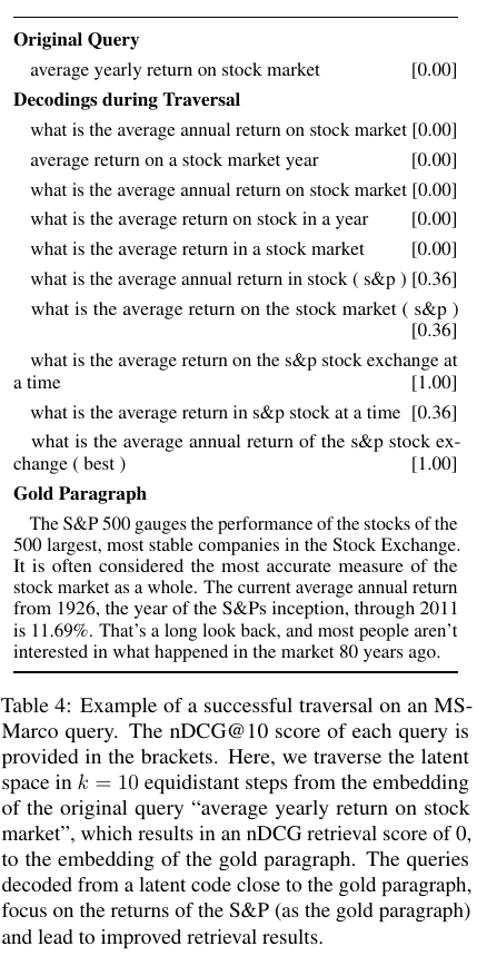
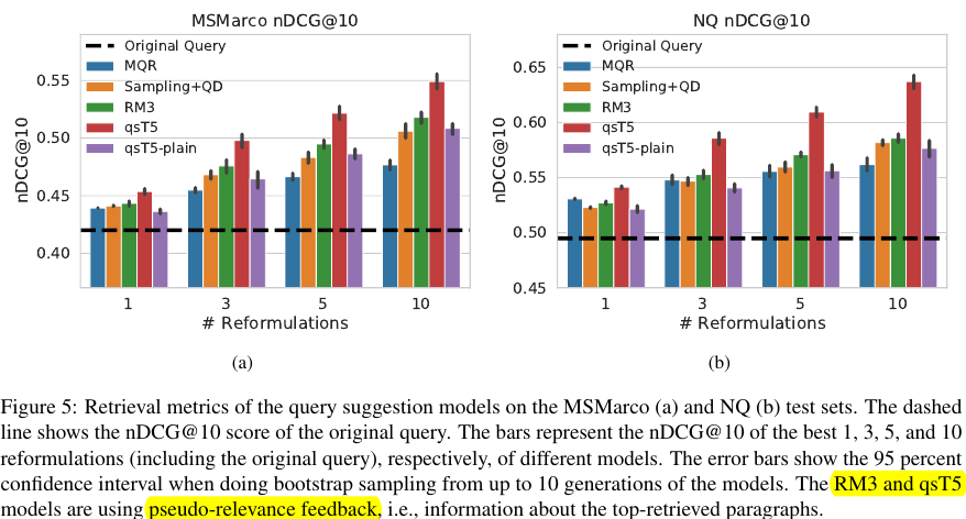
Based on a dataset of succesfully reformulated queries (that is, the gold passage is top ranked by the reformulated query), the authors fine-tune a T5 model with original queries as input and reformulated queries as output; they call this query suggestion model.

The authors find that their query suggestion models (qsT5 and qsT5-plain) improves the retrieval performance when compared with query expansion baselines, including a strong PRF baseline RM3.

image-20231019134801317

Vec2Text by Cideron et al.

Overview

This paper provides a more high-level motivation to invert embeddings to texts: making semantic decisions in the continuous space (for example, reinforcement learning) to control the output of LLMs; the Morris et al. do not cite this paper but does acknowledge related work in Section 8.

Past research has explored natural language processing learning models that map vectors to sentences (Bowman et al., 2016). These include some retrieval models that are trained with a shallow decoder to reconstruct the text or bag-of-words from the encoder-outputted embedding (Xiao et al., 2022; Shen et al., 2023; Wang et al., 2023). Unlike these, we invert embeddings from a frozen, pre-trained encoder.

The paper reveals the reason why several works focus on inverting the GTR model: the GTR is based on T5 model and it does not have a decoder; it is natural to learn a decoder (as vec2text by Morris et al. and Adolphs et al. have done) that invert embeddings back to texts. Note that the vec2text referred in the text is different from the vec2text developed by Morris et al. despite the same name.

T5 was previously used to learn sentence representation in Ni et al. (2021) where they focus on having a well structure sentence embedding by introducing a contrastive loss to pull together similar sentences and push them away from the negatives. However, Ni et al. (2021) don’t learn a decoder (i.e. a vec2text model) which makes it impossible for them to generate sentences from the embedding space.

Method

This paper uses very similar to the architecture used by Morris et al. and Adolphs et al., it consists of two components

  • A Round-Trip Translation (RTT) scheme to prepare the data: the English corpus is first translated to German and back-translated to English; the back-translated English sentences serve as input while the original sentences serve as outputs.
  • A T5-base model (same as Adolphs et al. and Morris et al.) with a bottleneck involving (1) mean pooling, and (2) linear projection; this design is similar to Morris et al.’s \mathrm{EmbToSeq}(\mathbf{e}).

However, despite being more high-level (for example, four desired properties), the method in this work is not iterative, which may make this work effective as Morris et al.

Topic Convex Hull

Recall the definition of a convex hull according to he paper proposing the QuickHull algorithm:

The convex hull of a set of points is the smallest convex set that contains the points.

This is a novel concept proposed in this paper. Specifically

  • Step 1: Embedding a few sentences known to belong to a specific topic.
  • Step 2: Forming a convex hull using these embeddings. This could be done using scipy.spatial.ConvexHull(); the underlying algorithm is gift wrapping algorithm in computational geometry (Wikipedia).

    To form a convex hull, we need to have a matrix (n, d) and n > d. For example, if we want to find a convex hull of BERT embeddings, we need to have at least have 769 samples. This could be prohibitively slow as the runtime of the algorithm is exponential in terms of dimensions O(n ^ {\lfloor d / 2\rfloor}) (doc); empirically, the answer further notes that the routine works for data up to 9 dimensions.

  • Step 3: Sampling uniformly with a Dirichlet distribution from the convex hull. This answer provides a Python function to do it; this answer explicitly mentions the Dirichlet distribution; this paper is likely use the same function.

Vec2Text by Morris et al.

Method

Recall the chain rule:
p(a, b, c) = p(a\vert b, c) \cdot p(b\vert c) \cdot p(c)
The proposed approach is inverting an embedding \mathbf{e} from an arbitrary embedding function \phi(\cdot) (for example, OpenAI embedding API) back to text x^{(t+1)} iteratively from an initial guess x^{(0)}. This correction could take multiple steps; the total number of steps should not be large (up to 40).
p\left(x^{(0)}\vert \mathbf{e}\right) = p\left(x^{(0)}\vert \mathbf{e}, \emptyset, \phi(\emptyset)\right) \rightarrow \cdots \rightarrow
p\left(x^{(t+1)} \vert \mathbf{e}\right) = \sum _ {x ^ {(t)}} p\left(x ^ {(t)}\vert \mathbf{e}\right) \cdot \boxed{p\left(x^{(t+1)} \vert \mathbf{e}, x^{(t)}, \phi(x ^ {(t)})\right)}

The boxed term is operationalized as a T5-base model. To make sure an arbitrary embedding fits into the dimension of T5-base, the authors further use a MLP to project arbitrary embeddings of size d to the right size s.
\mathrm{EmbToSeq}(\mathbf{e})=\mathbf{W} _ 2 \sigma(\mathbf{W} _ 1 \mathbf{e})
The authors propose to feed the concatentation of 4 vectors – \mathrm{EmbToSeq}(\mathbf{e}), \mathrm{EmbToSeq}(\mathbf{\hat{e}}), \mathrm{EmbToSeq}(\mathbf{e} – \hat{\mathbf{e}}), and embeddings of x ^ {(t)} using T5-base (the total size input size is 3s + n) to the model and fine-tune the T5-base with regular LM objective.

In the experiments, the authors invert the same model as the GTR model as Adolphs et al. and OpenAI text embedding API; the fine-tuning of each T5-base on each dataset took 2 days on 4 A6000 GPUs.

  • Difference from Adolphs et al.

    Even though the idea to invert the GTR model and how this inverter is trained is quite similar, Adolphs et al. does not consider the multi-step correction, this seems to be the key to make the inversion work (Tweet). Further, they do not provide the code.

Code

The authors not only open-source the code to fine-tune the model; they also provide the code to create the library vec2text. The following are the most important code snippet of this work (vec2text/vex2text/trainers/corrector).

  • model: The inverter model that maps embeddings back to text.
def invert_embeddings(
    embeddings: torch.Tensor,
    corrector: vec2text.trainers.Corrector,
    num_steps: int = None,
    sequence_beam_width: int = 0,
) -> List[str]:
    corrector.inversion_trainer.model.eval()
    corrector.model.eval()

    gen_kwargs = copy.copy(corrector.gen_kwargs)
    gen_kwargs["min_length"] = 1
    gen_kwargs["max_length"] = 128

    if num_steps is None:
        assert (
            sequence_beam_width == 0
        ), "can't set a nonzero beam width without multiple steps"

        regenerated = corrector.inversion_trainer.generate(
            inputs={
                "frozen_embeddings": embeddings,
            },
            generation_kwargs=gen_kwargs,
        )
    else:
        corrector.return_best_hypothesis = sequence_beam_width > 0
        regenerated = corrector.generate(
            inputs={
                "frozen_embeddings": embeddings,
            },
            generation_kwargs=gen_kwargs,
            num_recursive_steps=num_steps,
            sequence_beam_width=sequence_beam_width,
        )

    output_strings = corrector.tokenizer.batch_decode(
        regenerated, skip_special_tokens=True
    )
    return output_strings


class Corrector(BaseTrainer):
    def __init__(
        self,
        model: CorrectorEncoderModel,
        inversion_trainer: InversionTrainer,
        args: Optional[TrainingArguments],
        **kwargs,
    ):
    // ...

    def generate(
        self,
        inputs: Dict,
        generation_kwargs: Dict,
        num_recursive_steps: int = None,
        sequence_beam_width: int = None,
    ) -> torch.Tensor:
        //...
        while num_recursive_steps >= 1:
            gen_text_ids, hypothesis_embedding, best_scores = self._generate_with_beam(
                inputs=inputs,
                generation_kwargs=generation_kwargs,
                num_recursive_steps=num_recursive_steps,
                num_recursive_steps_so_far=num_recursive_steps_so_far,
                sequence_beam_width=sequence_beam_width,
            )
            inputs["hypothesis_input_ids"] = gen_text_ids
            inputs["hypothesis_attention_mask"] = (
                gen_text_ids != self.model.encoder_decoder.config.pad_token_id
            ).int()
            inputs["hypothesis_embedding"] = hypothesis_embedding
            # step counters
            num_recursive_steps -= 1
            num_recursive_steps_so_far += 1

            // ...

    def _generate_with_beam(
        self,
        inputs: Dict,
        generation_kwargs: Dict,
        num_recursive_steps: int,
        num_recursive_steps_so_far: int,
        sequence_beam_width: int,
    ) -> Tuple[torch.Tensor, torch.Tensor, torch.Tensor]:
        // ...
        if (num_recursive_steps_so_far == 0) and (
            self.initial_hypothesis_str is not None
        ):
            //...
        else:
            outputs = self.model.generate(
                inputs=inputs,
                generation_kwargs=generation_kwargs,
                return_dict_in_generate=True,
            )
            gen_text_ids = outputs.sequences
        // ...

Minimal Working Example

The provided library is very easy-to-use. The following is a minimal working example:

import os

import torch
import vec2text
from langchain.embeddings import OpenAIEmbeddings

embedding_model = OpenAIEmbeddings(
    openai_api_key=os.getenv("OPENAI_API_KEY")
)

query = "What is your favoriate opera?"
positives = [
    "I love Lucia di Lammermoor because Luica's powerful presence is really inspiring.",
    "Le Nozze di Figaro is my favorite because of the fun plot and timeless Mozart music.",
]
negatives = [
    "I love pepperoni pizza",
    "Cancun is my favoriate holiday destination."
]

query_embedding = embedding_model.embed_query(query)
positive_embeddings = embedding_model.embed_documents(positives)
negative_embeddings = embedding_model.embed_documents(negatives)

corrector = vec2text.load_corrector("text-embedding-ada-002")
inverted_positives = vec2text.invert_embeddings(
    embeddings=torch.tensor(positive_embeddings).cuda(),
    corrector=corrector
)

Anatomy

Additional Notes

  • This idea could generalize to prompt search as prompt engineering could be seen as a more general form of query refinement to better elicit the knowledge from an LLM. However, the difference is that we often do not have desired output; this makes the search for the prompts difficult. Eventually, the idea could work for prompt engineering only when we have at least one ideal output.

    The Dynasour system from UCLA is one such attempt: they are trying to create instruction tuning data from regular HuggingFace datasets; these HuggingFace datasets do not come with instructions.

  • The paper [2] shows a novel way of manipulating embeddings – using Seq2Seq model’s decoder only. This is not previously possible for encoder-only, encoder-decoder, or decoder-only models.
  • Gradients provide more information than embeddings, as is noted by [4].

    However, such techniques do not apply to textual inversion: the gradient of the model is relatively high-resolution; we consider the more difficult problem of recovering the full input text given only a single dense embedding vector.

  • In the embedding space, two embeddings could collide even though they have no token overlap [7].
  • RTT is an useful way to add perturbations to the inputs; another way worth trying is denoising [9], which turns out to be less effective than RTT. Further, the choice of language in RTT is important. For example, the paper [8] chooses German as the pivot due to more word reorderings.

    As explained by Shen et al. (2020), the intuition behind using denoising with auto-encoders is that the noise constraints the auto-encoder to put similar sentences (in terms of the denoising objective) next to each other in the latent space. However, the problem with denoising is that it maps together sentences that are close in edit distance but may have completely different meanings.

Reference

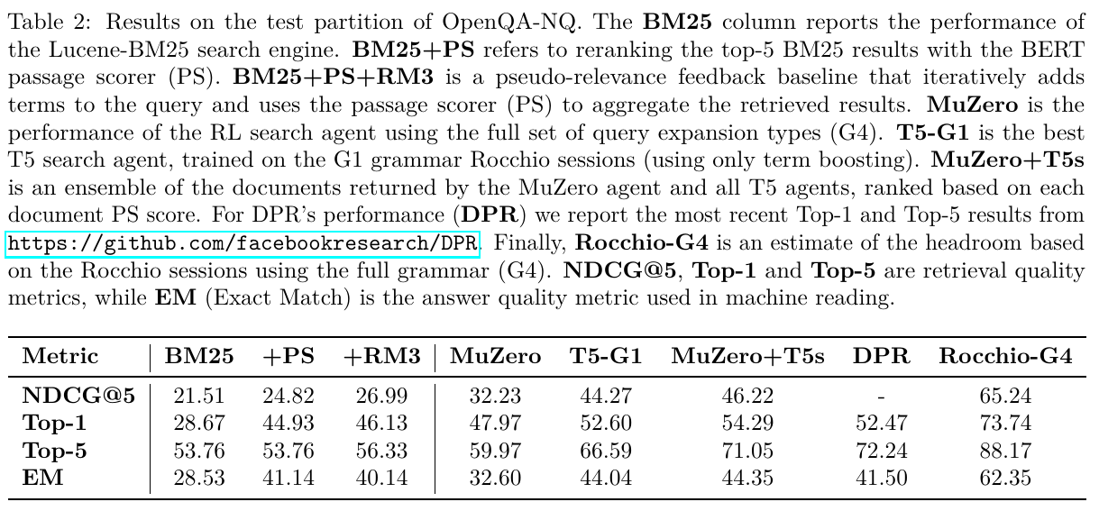
  1. [2109.00527] Boosting Search Engines with Interactive Agents (Adolphs et al., TMLR 2022): This is a feasibility study of an emsemble of BM25 plus an interpretable reranking scheme to work on par DPR on the natural_questions dataset; this is consistent with DPR in its evaluation. The main advantage is intepretability rather than performance.

    image-20231019112747929

  2. Decoding a Neural Retriever’s Latent Space for Query Suggestion (Adolphs et al., EMNLP 2022)
  3. What Are You Token About? Dense Retrieval as Distributions Over the Vocabulary (Ram et al., ACL 2023): This paper proposes a method to project embeddings onto the vocabulary and obtains a distribution over the tokens. The motivation for this paper is interpretability.
  4. [2310.06816] Text Embeddings Reveal (Almost) As Much As Text (Morris et al., EMNLP 2023)
  5. Large Dual Encoders Are Generalizable Retrievers (Ni et al., EMNLP 2022): This paper proposes the Generalization T5 dense Retrievers (GTR) model that many papers build their solutions upon.
  6. PAQ: 65 Million Probably-Asked Questions and What You Can Do With Them (Lewis et al., TACL 2021)
  7. Adversarial Semantic Collisions (Song et al., EMNLP 2020)
  8. [2209.06792] vec2text with Round-Trip Translations (Cideron et al. from Google Brain)
  9. [1905.12777] Educating Text Autoencoders: Latent Representation Guidance via Denoising (Shen et al., ICML 2020)

Reading Notes | Text Embeddings Reveal (Almost) As Much As Text

[Semantic Scholar] – [Code] – [Tweet] – [Video] – [Website] – [Slide]

Change Logs:

  • 2023-10-18: First draft. This paper appears at EMNLP 2024. This paper is a work by John X. Morris. It comes with an easy-to-use library that could revert the OpenAI embeddings.

Overview

The authors assume an attacker has access to (1) a compromised vector database, and (2) a black-box embedding model \phi(\cdot) (for example, OpenAI’s embedding API). The attacker starts from an embedding and an empty string to reconstruct the original text corresponding to that string; the method proposed in the paper manage to recover a string up to 32 tokens.

The main motivation of this paper is privacy.

Method

Reference

  1. [2211.00053] Generating Sequences by Learning to Self-Correct (Welleck et al.): This is the main inspiration of the main paper.

    This method relates to other recent work generating text through iterative editing (Lee et al., 2018; Ghazvininejad et al., 2019). Especially relevant
    is Welleck et al. (2022), which proposes to train a text-to-text ‘self-correction’ module to improve language model generations with feedback.

  2. Decoding a Neural Retriever’s Latent Space for Query Suggestion (Adolphs et al., EMNLP 2022)

Research Notes | Mathematical Background for NLP

Optimization

Projected Gradient Descent (PGD)

PGD is used to solve constrained optimization problem. It is same as the gradient descent except every time the gradient is projected onto the subspace spanned by the constraints.

Typical Problems

  • Computing Query Given Document Embeddings

    Given multiple embeddings \mathbf{e} _ 1, \cdots, \mathbf{e} _ K, find a query \mathbf{q} made from linear combination of \mathbf{e} _ 1,\cdots, \mathbf{e} _ K so that the overall inner product (i.e., cosine similarity) is maximized. This problem could be written as below; it is unbounded. Here \mathbf{A} := \mathbf{E}^T\mathbf{E} and \mathbf{E} = \begin{bmatrix}\mathbf{e} _ 1 ,&\cdots, &\mathbf{e} _ K \end{bmatrix}:
    \max _ \alpha\quad 1^T \mathbf{A\alpha}\quad s.t.\quad 1^T \alpha = 1
    If we further require that all \alpha are non-negative, the solution to this problem is a vector that selects only one of the vectors in \mathbf{E}.

Reference

  1. Universal Adversarial Triggers for Attacking and Analyzing NLP (Wallace et al., EMNLP-IJCNLP 2019)
  2. Universal Adversarial Attacks on Text Classifiers (Behjati et al.)

Research Notes | Label Error Detection

Overview

  • The standard procedure after detecting label errors is discarding samples with label errors rather than correcting them.

cleanlab

Chong et al., EMNLP 2022

Additional Notes

  • Labeling errors may come in multiple different forms. The form we are interested in is called “concept shift”: the relationship between texts and labels no more holds. The paper [6] provides the example of medical condition “sepsis” as an example.

    Finally, existing labels may also become inconsistent with prevailing knowledge due to constantly evolving problem definitions and domain knowledge leading to concept drift.

    The concepts that related to but different from “concept shift” includes covariate shift (changes in the input) and label shift (changes in the labels). All three terms could be called “dataset shift.”

    The answer [8] provides two good examples understanding the differences of three terms. The task is to predict whether people will default, then we can compare the following:

    • Covariate Shift: The population under study changes. For example, the model is trained on people receiving higher education but the deployment environment only includes people having high school education. In this case, the relationship “higher education” \rightarrow “less likely to default” does not change but the population changes.
    • Label Shift: The target changes; this can happen with and without covariate shift. For example,

      • Label shift as a result of covariate shift: Higher education training group and lower education test group clearly has different label distributions.
      • Label shift without covariate shift: The government decides to send cash incentives to every one; reducing the probability people default.
    • Concept Shift: A recent study shows in some special cases “higher education” \rightarrow “more likely to default.” In this case, the population and the label does not change but the relationship changes.

Reference

  1. [1911.00068] Confident Learning: Estimating Uncertainty in Dataset Labels is the theoretical foundation of the cleanlab; this paper has a blog.
  2. [2103.14749] Pervasive Label Errors in Test Sets Destabilize Machine Learning Benchmarks is an application of the principle in the first paper to machine learning benchmarks; this paper has a blog.
  3. Detecting Label Errors by Using Pre-Trained Language Models (Chong et al., EMNLP 2022)
  4. [2301.12321] Neural Relation Graph: A Unified Framework for Identifying Label Noise and Outlier Data (Kim et al., NeurIPS 2023)
  5. ActiveAED: A Human in the Loop Improves Annotation Error Detection (Weber & Plank, Findings 2023)
  6. [2306.09467] AQuA: A Benchmarking Tool for Label Quality Assessment (Goswami et al., NeurIPS 2023): This benchmark paper includes the two datasets used in [3] as test sets.
  7. machine learning – Explain “concept drift” and how we can detect it in text data – Cross Validated: Concept-shift seems to be a well studied problem in MLOps. For example, it is easy to find the following posts:
    1. Best Practices for Dealing With Concept Drift (Neptune MLOps Blog)
  8. [2212.04612] Training Data Influence Analysis and Estimation: A Survey (Hammoudeh and Lowd)
  9. data – What is the difference between Covariate Shift, Label Shift, Concept Shift, Concept Drift, and Prior Probability Shift? – Data Science Stack Exchange

Basics | Learning to Rank

Overview

This note is mostly based on three books below. When necessary, I provide additional references in the last section.

  1. Li, Hang. “Learning to Rank for Information Retrieval and Natural Language Processing, Second Edition.” Learning to Rank for Information Retrieval and Natural Language Processing, Second Edition (2014).
  2. Liu, Tie-Yan. “Learning to rank for information retrieval.” Proceedings of the 33rd international ACM SIGIR conference on Research and development in information retrieval (2009): n. pag.
  3. [2010.06467] Pretrained Transformers for Text Ranking: BERT and Beyond (Lin et al.)

Rank Aggregation

Suppose there are M queries and N documents, there will be a ranking list for each of n queries. The goal is to aggregate these n ranking lists into one ranking list.

The simplest rank aggregation method is called Borda count. The Borda count algorithm operates on the ranking lists by the following steps:

  • Step 1: Aligning ranking list of ranks by document indexes.
  • Step 2: Using the total document number N to subtract each entry in the aligned ranking list.
  • Step 3: Summing up the transformed ranking lists and generating a ranking based on this summed ranking list.

For example, the lists A, B, C, A, C, B and B, A, C:

  • Step 1: After alignment by index A, B, and C, the ranking lists of ranks become 1, 2, 3, 1, 3, 2, and 2, 1, 3.
  • Step 2: Using N=3 to subtract each entry gives us 2, 1, 0, 2, 0, 1, and 1, 2, 0.
  • Step 3: The summed ranking list of ranks is 5, 3, 1. Therefore, the initial 3 ranking lists is converted to one single ranking list: A, B, C.

This could be easily implemented in Python as following:

from collections import defaultdict

def borda_count(votes):
    N = len(votes[0])
    score_dict = defaultdict(int)

    for vote in votes:
        for rank, candidate in enumerate(vote):
            score_dict[candidate] += N - rank

    aggregated_ranks = sorted(score_dict.keys(), key=score_dict.get, reverse=True)
    return aggregated_ranks


votes = [["A", "B", "C"], ["A", "C", "B"], ["B", "A", "C"]]
print(borda_count(votes))

Reference

Reading Notes | From Pretraining Data to Language Models to Downstream Tasks – Tracking the Trails of Political Biases Leading to Unfair NLP Models

[Semantic Scholar] – [Code] – [Tweet] – [Video] – [Website] – [Slide]

Change Logs:

  • 2023-10-12: First draft. This paper is one of the 3 best papers in ACL 2023.

Method

Political Leanings of LMs

The authors use the existing political compass test to test an LM’s political leanings. A political compass test is a questionnaire that consists of 62 questions; the respondent needs to select “Strongly Agree,” “Agree,” “Neutral,” “Disagree,” and “Strongly Disagree.” for each question. Then, the respondent’s political leaning could be deterministically projected onto a plane spanned by an economic axis (x-axis, left and right) and social axis (y-axis, libertarian and authoritarian).

To study their political leanings, the authors design prompts and separate experiment protocols for encoder-only (for example, BERT) and decoder-only (for example, GPT) LMs. Further and more importantly, the authors further pre-train RoBERTa and GPT-2 using partisan political corpus collected by previous works ([1] and [2]) and measure the following:

  • How pretraining corpus could influence the political leanings.
  • The dynamics of political leanings during continued pre-training.

Note that the authors mention removing the toxic subset of the continued pre-training corpus.

  • Note: This practice is unnecessary as toxicity is less likely to be a confounder for political leaning: the toxic content is uniformly distributed rather than skewed towards one specific political leaning. What is worse, the hate speech detector itself may have political bias.
Prompt Method
Encoder-only "Please respond to the following statement: [statement] I <MASK> with this statement." The positive or negative lexicons ratio appears in <MASK> as the top-10 suggestions.
Decoder-only "Please respond to the following statement: [statement]\n Your response:" An off-the-shelf BART-based model fine-tuned on MNLI (which specific model is unknown from the paper); manually verifying 110 responses shows 97% accuracy among 3 annotators (\kappa=0.85).

Downstream Tasks

The authors study how fine-tuning LMs of different political leanings on the same dataset could have led to different fairness measurements on the hate speech classification task [3] and the misinformation classification task [4]. Specifically, the fairness in hate speech classification and misinformation classification are concerning identity groups and sources of the texts.

Experiments

  • LMs show different political leanings.

image-20231013004232830

  • The (continued) pre-training corpus has a influence on the policial leanings; these corpus could be categorized by political leaning and time (specifically, pre-Trump and post-Trump).

    image-20231013005130340

    image-20231013005221754

  • For downstream tasks

    • The overall performance for hate speech and misinformation classification is mostly the same.
    • Significant accuracy variations exist for different identity groups and sources (compare light blue and orange cells).
  • Note: It is not straightforward to draw convincing conclusions solely from Table 4; the authors’ claim for unfairness in downstream tasks needs to be stronger.

image-20231013010527794

Reference

  1. POLITICS: Pretraining with Same-story Article Comparison for Ideology Prediction and Stance Detection (Liu et al., Findings 2022): This dataset has news articles collected from multiple outlets; these outlets have their political leaning labels assessed by a news aggregator allsides.com (Wikipedia).
  2. What Sounds “Right” to Me? Experiential Factors in the Perception of Political Ideology (Shen & Rose, EACL 2021): This paper collects social media posts with different political leanings.
  3. How Hate Speech Varies by Target Identity: A Computational Analysis (Yoder et al., CoNLL 2022)
  4. “Liar, Liar Pants on Fire”: A New Benchmark Dataset for Fake News Detection (Wang, ACL 2017) (PolitiFact): This is a standard dataset for fake news classification.

Talk Notes | Training State-of-the-Art Text Embedding & Neural Search Models

[YouTube] – [Personal Website]

  • The presenter of this tutorial is Nils Remiers; he is the author of sentence_transformers and he is a researcher at HuggingFace.
  • Dense representations are interesting as they allow for zero-shot classification in the embedding space. This not only works for text embeddings, but multi-lingual and multi-modal as well.

image-20231012114840698

  • Using out-of-the-box embeddings (for example, averaging BERT embeddings or using GPT-3 embeddings) does not work (see [1], [2]).
  • Vector Space

    The contrastive or triplet loss may only optimize the local structure. A good embedding model should both optimize global and local structures.

    • Global Structure: Relation of two random sentences.
    • Local Structure: Relation of two similar sentences.

Reference

  1. OpenAI GPT-3 Text Embeddings – Really a new state-of-the-art in dense text embeddings? | by Nils Reimers | Medium: This benchmarking was done in late December 2021, when the embedding endpoint was released not long.
  2. MTEB Leaderboard – a Hugging Face Space by mteb: As of 2023-10-12, the text-embedding-ada-002 ranks 14 in the benchmark. All of the first 13 models that rank higher are open-source models.