Research Notes | Research Questions

Overview

Here I document a list of general research questions that warrants searching, reading, thinking, and rethinking.

General Topics

Model Capacity

  • What is the broadly applicable measure of model capacity similar to a hardware performance benchmark that helps practitioners pick up the suitable model to start building their applications?

    • Note: Model capacity mostly determines the performance upper bound of a model. The actual model performance may also related to how the model is trained with what set of hyperparameters.
    • Hypothesis: A straightforward choice is the number of parameters a model has. However, one may question the correlation between the parameter count and this measure, i.e., the parameter count may need to be a valid proxy for the model capacity.

Generalization

  • Existence of Universal Generalization

    Specifically, suppose there are K texts existing in the world at time t, and they are all labeled by an oracle; if we fine-tune a bert-base-uncased with k \ll K samples as a classification model, is there any hope that this fine-tuned model perform reasonably well (needs more precise definition) on all (K-k) samples.

    • Experiment: We could only approximate the oracle by some knowingly most capable models like GPT-4. We therefore have two datasets, one from (a) original annotations and (b) the other from oracle (approximated by GPT-4) annotations. Could the model fine-tuned on dataset (b) generalize better than (a)?
    • Question: Despite the generalization, could the fine-tuned model also inherit the bias (needs more precise definition) of GPT-4?

Text Classification, Annotation Bias, and Spurious Correlation

Does text classification work by relying on the spurious correlation (likely due to annotation bias where the annotators seek to take the shortcuts to complete their assigned tasks as soon as possible) between a limited number of words in the input text and output label? Therefore, is the better model indeed the model that better exploits the spurious correlation?

> - Hypothesis: If the K samples are all annotated by an oracle, then any *reasonably capable* model (needs more precise definition) can generalize well. 
> - Tentative Experiment: If we replace the words in the list with their hypernyms, will the system performance drop?

Life Long and Continual Learning

Suppose we have a generalizable model at time t if we want the model to serve the users indefinitely. What are the strategies that make the model generalize well across time?

Data Distribution

In machine learning theory, we often encounter concepts such as “i.i.d.” Understanding “distribution” for tabular data is straightforward, where the list of variables forms a joint distribution that predicts the label y. However, what could be considered a “distribution” for texts is less clear. Note that this is possible for images, for example, modeling the gray-scale images as a Dirichlet multimodal distribution that predicts digits from 0 to 9.

Data Annotation

The labels in the NLP tasks have different levels of subjectivity. For example, the grammatical error correction is less subjective, sentiment classification is moderately subjective, and the topics like hate speech, suicidal ideation [1], and empathy [2] are either extremely subjective or requires expert knowledge.

The difficulty here it to mitigate the ambiguity during data annotation and make sure the information available in texts matches well with the label. Ideally, if we know the true underlying label of a text, we could fine-tune any reasonably capable model to generalize well.

Data Selection and Data Pruning for Classification Tasks

As of 2023-10-11, I have not seen a single work on the data selection for classification tasks; there are plenty of works on optimizing data mixture for language model pretraining. One likely reason why this happens is that the quality of classification datasets depends on both texts and labels; investigating the label quality is hard.

Special Issues

Improving Machine Learning Models with Specifications

The difference of testing machine learning models versus testing traditional software is that the action items for the latter is generally known after testing and could be executed with high precision, while for the former, we do not know how we will improve the model.

Suppose the model could already achieve high accuracy on the standard test set (it is indeed the train-to-train setting if we follow the WILDS paper), which means the model architecture, training objective, and hyperparameters are not responsible for the lower performance on the artificially created challenging set, the most straightforward way to improve the model performance is data augmentation. The naive way is to blindly collect more data that are wishfully relevant as an augmentation so we expect the performance could improve.

Guided Data Augmentation

However, this blindness hampers the efficiency of improving the models: the only feedback signal is the single scalar (i.e., failure rate) after we have trained and evaluated the model; we should have a feedback signal before we train the model.

  • Unverified Hypothesis: the feedback signal is highly (inversely) correlated with the failure rate on the benchmark.

Formally, we have a list of specifications in the format of (s_1, D _ 1, D _ 1 ^ \text{heldout}), (s _ 2, D _ 2, D _ 2 ^ \text{heldout}), \cdots, the model \mathcal{M}_0 trained on D _ \text{train} does well on D _ \text{train} ^\text{heldout} but poorly on D _ 1 \cup D _ 2 \cup D _ 3 \cdots as indicated by failure rate \mathrm{FR}. We additionally have a new labeled dataset D _ \text{unused}. The goal is to sample D _ \text{unused} using (s_1,D _ 1 ^ \text{heldout}), (s _ 2, D _ 2 ^ \text{heldout}), \cdots: \mathrm{Sample}(D _ \text{unused}); we also have a random sample with same size \mathrm{RandomSample}(D _ \text{unused}) as baseline.

  • Note: The D _ i and D _ i ^ \text{heldout} are completely different. For example, if the specification s _ i is operationalized through templates, these two sets are disjoint in terms of templates. What we are certain about D _ i and D _ i ^ \text{heldout} is that they are ideally sufficient and necessary with respect to s _ i; practically, the semantic underspecification of them are low [3].

There are a lot of things we could do with \mathrm{RandomSample}(D _ \text{unused}) and \mathrm{Sample}(D _ \text{unused}). For example

  • Fine-tuning a model from scratch using \mathrm{RandomSample}(D _ \text{unused}) \cup D _ \text{train}.
  • Patching the model using constrained fine-tuning [4] and related approaches.

Whichever method we choose, if we denote the intervention with \mathrm{RandomSample}(D _ \text{unused}) as \mathcal{M} _ 1 and \mathrm{Sample}(D _ \text{unused}) as \mathcal{M} _ 2. We expect the following conditions will hold:

  • $D _ \text{train} ^ \text{heldout}$: $\mathcal{M} _ 0 \approx \mathcal{M} _ 1 \approx \mathcal{M} _ 2$.
  • $D _ 1 \cup D _ 2 \cup D _ 3 \cdots$: $\mathcal{M} _ 2 \ll \mathcal{M} _ 0$, $\mathcal{M} _ 2 \ll \mathcal{M} _ 1$. That is, the specification-following data selection improves over the random selection on the specification-based benchmarks.
  • Assumption: The samples x _ {ij} is fully specified by the specification s _ i.
  • Note: If the annotations of a dataset strictly follow the annotation codebook, then the machine learning learns the specifications in the codebook. The process described above is a reverse process: we have a model that is already trained by others; we want to use the model in a new application but do not want to or can not afford to relabel the entire dataset, what is the minimal intervention we could apply to the dataset so that the model could quickly meet my specifications?

Detecting Inconsistent Labels with Specifications

Following the previous problem setup, we have a list of specifications in the format of (s_1, D _ 1, D _ 1 ^ \text{heldout}), (s _ 2, D _ 2, D _ 2 ^ \text{heldout}), \cdots; each specification has an unambiguous label. Rather than augmenting the D _ \text{train} with additional data by selecting using either (1) D _ 1 ^ \text{heldout} \cup D _ 2 ^ \text{heldout} \cup \cdots itself or (2) a model trained on it, we aim to correct labels directly in D _ \text{train} which are inconsistent with specifications.

Specifically, we could do the following for train, validation, and test sets:

  • Note: It is important to note that the data splitting should happen before we correct labels; otherwise the scores between trials will not be comparable. An alternative is to use D _ 1 ^ \text{heldout} \cup D _ 2 ^ \text{heldout} \cup \cdots as the validation set so that all scores are comparable.
  • Step 1: Grouping the specifications by the binary labels (for example, 0 and 1).
  • Step 2: Using the queries corresponding to each label to rank samples D _ s; each sample in D _ s will receive an integer ranking ranging from 0 to \vert D _ s \vert. For example, for a set of positive specifications S^+, his will lead to a matrix of shape (\vert D _ s\vert, \vert S^+ \vert).
  • Step 3: Merging the \vert S^+\vert (or \vert S^-\vert) ranking list into one list using some rank aggregation methods.
  • Step 4: Removing all samples of label 0 (or 1). The top-k samples are the ones that should be corrected.

The main issue with this pipeline is that the number of corrected samples is strictly no more than k; retraining with only \frac{k}{\vert D _ \text{train}\vert} of labels changed may not have direct impact on the modified model.

  • Note: This process is different from cleanlab as the latter does not consider specifications (i.e., the guaranteed uncorrupted labels). Their setting is useful in many ways as their system only require noisy labels and predicted probabilities of each sample.

Reverse Engineering Queries Given Documents

For a DPR model trained on large corpus (for example, facebook/dpr-ctx_encoder-single-nq-base and facebook/dpr-question_encoder-single-nq-base), if we have a list of documents D that are aligned with our goal (or true underlying query) q, is it possible to search for its approximated version \hat{q} that returns D as relevant documents with high probability?

A somehow related problem called Doc2Query has been studied before; the difference is that these previous works use Doc2Query as a data augmentation (it is called document expansion in the IR community) approach.

With the vec2text, it may be possible to search for the best query in the embedding space using approaches like Projected Gradient Descent (PGD).

Geometry of Embeddings and its Implication for Text Generation

This is based on the hypothesis that there exists certain relation between the geometry of embedding space and semantic meaning of each point in that space. For example, sampling a convex set leads to sentences that have similar high-level specifications.

Many recent works show that text embeddings may be anisotropic: directions of word vectors are not evenly distributed across space but rater concentrated in a narrow cone; this peculiarity may not be related to performance [7].

Retrieval Augmented LM

RALM could be useful in numerous ways.

  • Copyright: This is the idea of SiloLM, where the LM itself is fine-tuned with CC0 data. The copyright data is stored in a non-parametric database; these data could be incorporated into the inference process using RALM. However, with this design, the authors of the copyrighted texts could easily request a removal.
  • Traceability: The retrieved samples serve as evidence to support the decisions made by the LM.
  • QA: When we would like to do QA on a large tabular database (for example, asking “what is the percentage of patients who have allergy” to a large EHR database), the RALM is the most natural way to incorporate the necessary information in the database into the inference process of an LLM. Previously we need to build a pipeline that first generates queries written in formal language (for example, ElasticSearch queries) and then use these generated queries to answer the question.

These benefits are offered by the complementary nature of non-parametric databases’ high data fidelity and LMs’ inference ability. Specifically, the knowledge is stored distributionally in the LM; it is not straightforward to retrieve the exact know compared to using a non-parametric database. At the same time, the inference ability available to exploit in LMs are not available in other smaller models.
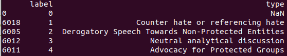
HateModerate

  • Dataset Statistics

image-20231107125236836

Label Inconsistency of Different Datasets

Given multiple datasets D_1, D_2, \cdots with the same input and output space \mathcal{X} \times \mathcal{Y} (for example, binary hate speech classification), is there a systemic approach that finds inconsistent labeling criteria. Specifically, if two similar sentences that belong to two datasets receive different labels, how do we explain the discrepancy in their underlying labeling criterion? This is done preferably in the format of FOL or natural language.

  • If we treat GPT-4 as an oracle and use it to annotate the samples from D _ 1, D _ 2, \cdots, we could obtain an accuracy vector of size \vert \mathcal{Y} \vert to characterize the label quality of each dataset. Note that for comparison purposes, the datasets to be annotated should be made same size and remains the original label distribution.

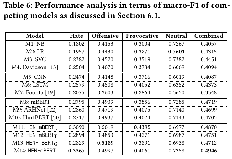
    Previously it has been shown that using a simple zero-shot prompt shows an binary label inconsistency rate from 9% to up to 36%; the datasets under study are 15 hate speech datasets (uniform random sample of 200 samples per dataset) whose labels have been normalized to binary labels per each dataset’s description.

    Note: The dataset label normalization process may be questionable.

Adversarial Attack on RLHF

We assume there is an underlying utility function U: \mathcal{Y} \rightarrow [-1, 1] that measures a response y‘s alignment to the input x: a response receives a high score when it is helpful, honest, and harmless.

  • One thing we could do is investigating the relation between the ratio of reversed comparison pairs and the degradation on performance on the downstream tasks, such as HHH.
  • The comparison reversal is not uniformly adversarial to the downstream tasks. If U(y _ i) and U(y _ j) is very close, then reversing them is not as effective as reversing another pair where U(y _ i’) and U(y _ j ‘) is very different.

OOD for Reward Model in RLHF

The reward model r(x, y; \phi) is fixed when fine-tuning the LM with PPO. There may be some distribution shifts between two stages. From the high level, this may not be an issue as the goal of RLHF is general enough (for example, HHH and Constitutional AI).

Applications of RLHF to Other Tasks

According to Hyungwon Chung, RLHF is the new paradigm to create application-specific loss function. It is therefore likely beneficial to abandon traditional cross-entropy loss altogether and opt for RLHF.

Pairwise Regression

This is especially useful for highly abstract tasks like hate speech classification. For example, we could initialize a RM and use the normalized score [0, 1] (for example, hatefulness) to fine-tune a hate speech regressor based on some open-source models. We could find a threshold on the validation set and then deployment the RM (with a threshold) to the testing environment. This idea is indeed the pairwise regression; it is one of three approaches (point-wise, pairwise, and list-wise) for learning to rank.

References

  1. ScAN: Suicide Attempt and Ideation Events Dataset (Rawat et al., NAACL 2022)
  2. A Computational Approach to Understanding Empathy Expressed in Text-Based Mental Health Support (Sharma et al., EMNLP 2020)
  3. Dealing with Semantic Underspecification in Multimodal NLP (Pezzelle, ACL 2023)
  4. [2012.00363] Modifying Memories in Transformer Models (Zhu et al.)
  5. cleanlab

    1. [1911.00068] Confident Learning: Estimating Uncertainty in Dataset Labels is the theoretical foundation of the cleanlab; this paper has a blog.
    2. [2103.14749] Pervasive Label Errors in Test Sets Destabilize Machine Learning Benchmarks is an application of the principle in the first paper to machine learning benchmarks; this paper has a blog.
  6. Doc2Query

    1. [1904.08375] Document Expansion by Query Prediction (Nogueira et al.)
    2. From doc2query to docTTTTTquery (Nogueira and Lin) and its associated GitHub.
    3. [2310.06816] Text Embeddings Reveal (Almost) As Much As Text (Morris et al., EMNLP 2024)
    4. Decoding a Neural Retriever’s Latent Space for Query Suggestion (Adolphs et al., EMNLP 2022)
  7. Is Anisotropy Truly Harmful? A Case Study on Text Clustering (Ait-Saada & Nadif, ACL 2023)

Reading Notes | Exploring and Predicting Transferability across NLP Tasks

[Semantic Scholar] – [Code] – [Tweet] – [Video] – [Website] – [Slide]

Change Logs:

  • 2023-09-16: First draft. This paper appears at ACL 2020.
  • Data selection strategy for best transfer learning performance.

Reference

  1. [1811.01088] Sentence Encoders on STILTs: Supplementary Training on Intermediate Labeled-data Tasks (Phang et al)
  2. Identifying beneficial task relations for multi-task learning in deep neural networks (Bingel & Søgaard, EACL 2017)

Talk Notes | Lessons Learned from Analyzing Systems for Hate Speech Detection and Bias Mitigation by Sarah Masud

[YouTube] – [Personal Website]

  • The presenter has authored several interesting papers ([1] through [5]) on hate speech detection.

Notes

Status Quo of Hate Speech Detection

  • There are varying definitions of hate speech.
  • Labels related to hate speech include hate, offensive, toxic, profane, and toxic. There could be also more fine-grained categories, such as sexist, racist, and islamophobic.
  • Because of the reasons mentioned above, there is no leaderboard in hate speech detection.

Data Sources

We should pay attention to data bias; it is doubtful to collect hate speeches from people and sites that are more likely to generate hate speech. The authors propose to collect datasets from neutral sources; this design choice makes the data annotation difficult.

Annotations

Current approaches of hate speech annotation rely on people (crowdworkers or experts). The authors use the two-phase approach to ensure the label quality.

Building Better Hate Speech Detection Models

  • The complexity of models does not necessarily help. It is more important to capture the signals that predict the final labels, for example, the history and the social network information. This observation also applies to other tasks that involve modeling social behaviors.
  • However, we should carefully monitor the overfitting: spurious correlation between overfitted phrases and labels should not be the signals we allow the models to pick up. That is, the models should generalize without the presence of these words.
  • In the work [2], the authors propose a system that considers not just the text information, but also the timeline and social network information. They merge the three sources of signal using an attention mechanism. However, we could see two limitations:
    • This design is specific to Twitter. Other platforms, such as Reddit, do not have this information with respect to users.
    • The best performing system (M14) does not significantly outperform the baseline system, which is simply fine-tuning a mBERT (M8).

image-20230925174150642

Lexical Bias

  • Replacing the bias sensitive words with more general words is likely shift the bias towards the WordNet ancestors. This hypothesis could be supported by a measurement called pinned bias, where t is the single word in the sensitive word list.

pB _ T = \sum _ {t \in T} \frac{\vert p(\text{“toxic”}\vert t) – \phi\vert}{ \vert T \vert},\quad \phi=\min(p(\text{“toxic”}\vert t), 0.5)

Horizons

The presenter has three high-level observations:

  • Like energy: Bias seems to be transferring from one source to the other.
  • Like a system at rest: A model or dataset will remain biased unless external force (for example, mitigation and regularization) is enabled.
  • Like interactive systems: A system is evolving more chaotic over time. The toxicity needs to be monitored and mitigated in a continuous fashion.

Reference

  1. [2010.04377] Hate is the New Infodemic: A Topic-aware Modeling of Hate Speech Diffusion on Twitter (Masud et al., ICDE 2021): This paper presents a dataset called RETINA that focus on hate speech in the Indian context.
  2. [2206.04007] Proactively Reducing the Hate Intensity of Online Posts via Hate Speech Normalization (Masud et al., KDD 2022)
  3. [2201.00961] Nipping in the Bud: Detection, Diffusion and Mitigation of Hate Speech on Social Media (Chakraborty and Masud)
  4. [2306.01105] Revisiting Hate Speech Benchmarks: From Data Curation to System Deployment (Masud et al., KDD 2023)
  5. [2202.00126] Handling Bias in Toxic Speech Detection: A Survey (Garg et al., CSUR).
  6. Language (Technology) is Power: A Critical Survey of “Bias” in NLP (Blodgett et al., ACL 2020)
  7. [2305.06626] When the Majority is Wrong: Modeling Annotator Disagreement for Subjective Tasks (Fleisig et al.)
  8. Handling Disagreement in Hate Speech Modelling | SpringerLink (Novak et al., IPMU 2022)
  9. [2001.05495] Stereotypical Bias Removal for Hate Speech Detection Task using Knowledge-based Generalizations (Badjatiya et al., WWW 2019).

Reading Notes | Revisiting Hate Speech Benchmarks – From Data Curation to System Deployment

[Semantic Scholar] – [Code] – [Tweet] – [Video] – [Website] – [Slide]

Change Logs:

  • 2023-09-21: First draft. This paper appears at KDD 2023. The co-lead author – Sarah Musud – has published numerous papers on hate speech detection.

Additional Notes

  • Measuring Dataset Difficulty

    The authors compare different datasets’ difficulty using the JS divergence between Laplician smoothed unigram distributions of texts under different label pairs; the lower the divergence, the closer the unigram distributions and this makes texts under a label pair more difficult to distinguish.

    For example, the proposed datasets have 4 labels, this will lead to \binom{4}{2} = 6 divergence measures.

  • Matthews Correlation Coefficient (MCC)

Reference

Coding Notes | HuggingFace Reference

Basics

Hyperparameters

  • The hyperparameters are specified through TrainingArguments and Seq2SeqTrainingArguments.
  • model_name_or_path and output_dir are the only two required arguments. However, we should also set other critical hyperparameters, including num_train_epochs, per_device_train_batch_size, per_device_eval_batch_size, learning_rate.

Evaluation, Logging, and Saving

  • It is better to set logging_steps to 1 and logging_strategy to step as logging is beneficial whatsoever yet does not cause significant overhead.
  • It is better to specify eval_steps as 1 / n and eval_strategy to "steps", where n is number evaluations. This will help collect enough samples even if we have fewer training steps or training epochs.
  • load_best_model_at_end=True has to pair with the following configurations (answer). It will save the best checkpoints according to the evaluations done throughout the training process:
    • After setting eval_steps to a decimal number, save_strategy has to be set to "steps" since save_steps has to be multiple of eval_steps. As saving larger models will take long time, we need to set save_steps to a reasonable number. For example, if we would like to evaluate the model for 10 times (i.e., eval_steps is set to 0.1), we should save twice (i.e., save_steps is set to 0.5).
    • save_total_limit governs the saving of the latest models; it is likely to save k+1 checkpoints even if save_total_limit=k as the best model is not the latest k models saved.
    • compute_metric has special syntax to follow. For example, the following is taken from the official run_glue.py. Here p.predictions depends on the specific model.
# You can define your custom compute_metrics function. It takes an `EvalPrediction` object (a namedtuple with a
# predictions and label_ids field) and has to return a dictionary string to float.
def compute_metrics(p: EvalPrediction):
    preds = p.predictions[0] if isinstance(p.predictions, tuple) else p.predictions
    preds = np.squeeze(preds) if is_regression else np.argmax(preds, axis=1)
    result = metric.compute(predictions=preds, references=p.label_ids)
    if len(result) > 1:
        result["combined_score"] = np.mean(list(result.values())).item()
    return result
Index Hyperparameter Value
1 save_strategy, eval_strategy steps or epoch; they have to be same.
2 eval_steps A reasonable value such as 0.1.
3 save_steps Must be the multiples of the eval_steps.
4 metric_for_best_model and compute_metric metric_for_best_model defaults to loss (or eval_loss with an automatically prepended eval_). It could be set to other custom metrics defined in compute_metric
  • It is recommended to use wandb. In order to do so, we need to set report_to and run_name. Note that if we need to use custom name on wandb portal, we should not rename the default output directory.

Testing Training Scripts

Index Hyperparameter Value Notes
1 max_train_samples, max_eval_samples, max_test_samples 100
2 save_strategy no
3 load_best_model_at_end False

Checkpoints

If a model has been fine-tuned, then most likely there will be only updates in pytorch_model.bin file. We could reuse the original config.json and the tokenizer.

  • A runnable model only consists of a pytorch_model.bin and a config.json file. The config.json documents the metadata of the model.
  • A tokenizer consists of a list of files:

    bash
    tokenizer/
    ├── added_tokens.json
    ├── merges.txt
    ├── special_tokens_map.json
    ├── tokenizer_config.json
    ├── tokenizer.json
    └── vocab.json

However, if we save checkpoints during training, then the code of saving checkpoints has already been taken care of.

Inference

langchain, Pipeline, and Model Classes

The classes and methods provided inmodel.generate() ,pipeline (or TextGenerationPipeline) and langchain are increasingly more high-level: the TextGenerationPipeline internally calls model.generate() and langchain.llms.huggingface_pipeline.HuggingFacePipeline internally uses TextGenerationPipeline.

Therefore, it is sufficient to understand how model.generate() works and how the more abstract classes wrap the other classes. See the following example. Note that

  • A better way to specify arguments is not through a dictionary but through a predefined class such as transformers.GenerationConfig and then model.config = config. This could make the most use of the code reference feature available in PyCharm.
  • We should stick to transformers.pipeline rather than TextGenerationPipeline as the former has the unified API across different tasks.
  • Here is the decision flow of which API to use:

    Index API Case
    1 model.generate() When we need special control over the outputs. For example, adding human bias to the distribution similar to logit_bias for OpenAI APIs (example) or transformers.NoBadWordsLogitProcessor.
    2 transformers.pipeline Preferred as the first choice.
    3 langchain When working with langchain
import os

os.environ["CUDA_VISIBLE_DEVICES"] = str(0)
os.environ["TOKENIZERS_PARALLELISM"] = "false"

import torch
from transformers import (
    pipeline,
    AutoTokenizer,
    AutoModelForCausalLM,
)
from langchain.llms.huggingface_pipeline import (
    HuggingFacePipeline,
)

##################################################

model = AutoModelForCausalLM.from_pretrained("gpt2")
tokenizer = AutoTokenizer.from_pretrained("gpt2")

prompt = "Great changes have taken place in the past 30 years"

##################################################
# method 1
# BAD: requires manually moving model and data to the device

config = {
    "do_sample": True,
    "top_p": 1,
    "num_return_sequences": 5,
    "temperature": 1,
    "max_new_tokens": 16,
}

device = torch.device("cuda:0")
model = model.to(device)
tokenizer.pad_token = tokenizer.eos_token

raw_response1 = model.generate(
    **tokenizer(prompt, return_tensors="pt").to(device),
    **config,
).squeeze()

texts1 = tokenizer.batch_decode(raw_response1)

##################################################
# method2
# GOOD

config = {
    "do_sample": True,
    "top_p": 1,
    "num_return_sequences": 5,
    "temperature": 1,
    "max_new_tokens": 16,
    "device": "cuda:0"
}

pipeline = pipeline(
    "text-generation",
    model=model,
    tokenizer=tokenizer,
    **config
)

response2 = pipeline(prompt)
texts2 = [response["generated_text"] for response in response2]

##################################################
# method 3
# GOOD: However, it could NOT generate multiple sequences at the same time

llm = HuggingFacePipeline(pipeline=pipeline)
texts3 = list()
for _ in range(5):
    texts3.append(llm(prompt))

Controlled Generation

Enforcing or Forbidding Specific Tokens

This is done using disjunctive constraints (enforcing) or NoBadWordsLogitsProcessor (forbidding) internally in model.generate(). This could be easily implemented using the snippet below.

Note that when enforcing generation, setting num_beams to an integer greater than 1 is critical as enforcing presence of some tokens is implemented using beam search.

from transformers import AutoTokenizer, AutoModelForCausalLM

def get_tokens_as_list(model_name, word_list):
    tokenizer_with_prefix_space = AutoTokenizer.from_pretrained(model_name, add_prefix_space=True)
    tokens_list = []
    for word in word_list:
        tokenized_word = tokenizer_with_prefix_space([word], add_special_tokens=False).input_ids[0]
        tokens_list.append(tokenized_word)
    return tokens_list


model = AutoModelForCausalLM.from_pretrained("gpt2")
tokenizer = AutoTokenizer.from_pretrained("gpt2")
tokenizer.pad_token_ids = tokenizer.eos_token_id

prompt = "Great changes have taken place in the past 30 years"

inputs = tokenizer(prompt, return_tensors="pt")
output_ids = model.generate(inputs["input_ids"], max_new_tokens=5)
print(tokenizer.batch_decode(output_ids, skip_special_tokens=True)[0])

words_ids = get_tokens_as_list(model_name="gpt2", word_list=["Donald", "Trump"])

output_ids = model.generate(inputs["input_ids"], max_new_tokens=5, bad_words_ids=words_ids)
print(tokenizer.batch_decode(output_ids, skip_special_tokens=True)[0])

output_ids = model.generate(inputs["input_ids"], max_new_tokens=5, force_words_ids=words_ids, num_beams=10)
print(tokenizer.batch_decode(output_ids, skip_special_tokens=True)[0])

Inference on Multiple Devices

It does not seem to easily make inferences on multiple devices. However, we could use optimized attention implemented torch>=2.0.0 and optimum to reduce the time and space requirement.

Instruction Tuning

Using the Basic transformers Library

It is possible to instruction-tune a language model using the official example script run_clm.py working with gpt2 or the Phil Schimid’s blog working with google/flan-t5-xl.

Using the trl Library

SFTTrainer() provided in the trl provides an another layer of abstraction; this makes instruction-tuning even easier and cleaner. However, the downsides are (1) it could not work well with deepspeed, and (2) it does not support everything (for example, setting save_steps to a decimal number) defined in transformers.TraingingArguments; this limits its flexibility.

  • Tuning a Model with the Language Modeling Objective

    This could be done in fewer than 14 lines of code. For example, tuning an LM on the imdb dataset. We could add more configurations to the code skeleton below (for example, PEFT, 4-bit / 8-bit) following the example script here.

from datasets import load_dataset
from transformers import AutoModelForCausalLM
from trl import SFTTrainer

dataset = load_dataset("imdb", split="train")
model = AutoModelForCausalLM.from_pretrained("facebook/opt-350m")

trainer = SFTTrainer(
    model,
    train_dataset=dataset,
    dataset_text_field="text",
    max_seq_length=512,
)
trainer.train()
  • Tuning a Model using the Completions – Self-Instruction

Tuning Large Models with Constrained Hardware

Overview

We have the following decision matrix when we are working on the single node; there may be other considerations when working with multiple nodes; a node means a machine’s GPUs are physically connected.

Single GPU Multiple GPUs
Mode Fits into Single GPU DDP
ZeRO (may or may not be faster)
Model Does not Fit into Single GPU ZeRO + Offload CPU + MCT (optional) + NVMe (optional) PP (preferred) if NVLink or NVSwitch is not available
ZeRO
TP
Largest Layer Does not Fit into Single GPU ZeRO + Offload CPU + MCT + NVMe (optional) TP
ZeRO + Offload CPU + MCT + NVMe (optional)
  • One single 7B LLaMA model is already almost 30 GB on HuggingFace; the 13B version will be even larger.
  • When using custom training loops. The accelerate library improves pytorch.distributed and makes it possible that the same code could be run on any hardware settings without making updates to the code.

    When using Trainer(), all of the distributed training settings could be done without using accelerate.

  • ZeRO is implemented using deepspeed.

Using a Single GPU

  • A typical model with AdamW optimizer requires 18 bytes per parameter.
  • Besides the methods described below, one could try accelerate library to use same torch code for any hardware configuration (CPU, single GPU, and multiple GPUs).
  • Besides the methods described below, one could try accelerate library to use same torch code for any hardware configuration (CPU, single GPU, and multiple GPUs).
Method Speed📈 Memory📉 Note
Batch Size Yes Yes It should be default to 8. But choosing a batch size that makes most of GPUs is complicated.
Dataloader Yes No Always set pin_memory=True andnum_workers=4 (or 8, 16, …) when possible.
Optimizer Yes Yes Using Adafactor saves 50% compared to Adam or AdamW. But it does not converge fast. This is supported out-of-box.
One could alternatively use 8-bit AdamW to save more than 50% memory when bibsandbytes is installed and used.
Gradient Checkpointing No Yes Supported by Trainer(..., gradient_checkpointing=True, ...).
Gradient Accumulation No Yes Supported by Trainer(..., gradient_accumulation_steps=4,...).
Mixed Precision Training Yes No fp16 is supported in TrainingArguments(.., fp16=True, ...).
With Ampere GPUs such as A100 or RTX-3090, bf16=True or tf32=True (with torch.beakends.cuda.mamul.allow_tf32=True) could be set.
DeepSpeed ZeRO No Yes The model with the smallest batch size does not fit into the GPU. Using Trainer() is supported out-of-box.

We could use the code below to measure the GPU utilization:

from pynvml import *

def print_gpu_utilization():
    nvmlInit()
    handle = nvmlDeviceGetHandleByIndex(0)
    info = nvmlDeviceGetMemoryInfo(handle)
    print(f"GPU memory occupied: {info.used//1024**2} MB.")

For example, when tuning a bert-large-uncased model with some dummy data, we could see on top of the following vanilla code:

  • Vanilla Code to Tune a Classification Model
import os
os.environ["CUDA_VISIBLE_DEVICES"] = str(0)

import numpy as np

from datasets import Dataset
from transformers import (
    Trainer,
    logging,
    TrainingArguments,
    AutoModelForSequenceClassification,
)

from utils.common import print_gpu_utilization

##################################################
logging.set_verbosity_error()

dataset_size, seq_len = 512, 512
train_dataset = Dataset.from_dict(
    {
        "input_ids": np.random.randint(100, 30000, (dataset_size, seq_len)),
        "labels": np.random.randint(0, 1, dataset_size),
    }
)
train_dataset.set_format("pt")
print_gpu_utilization()

##################################################

default_args = {
    "output_dir": "tmp",
    "evaluation_strategy": "steps",
    "num_train_epochs": 1,
    "log_level": "error",
    "report_to": "none"
}

training_args = TrainingArguments(
per_device_train_batch_size=4,
    **default_args
)

model = AutoModelForSequenceClassification.from_pretrained("bert-large-uncased").to("cuda")
print_gpu_utilization()

trainer = Trainer(
    model=model,
    args=training_args,
    train_dataset=train_dataset
)
result = trainer.train()

After making updates to the vanilla code, we could see the changes in the memory usage.

Basic Setup Memory (MB)
Loading Dummy Data 2631
Loading Model with per_device_train_batch_size=4 14949
Loading Model with per_device_train_batch_size=4 + 8-bit Adam 13085
Loading Model with per_device_train_batch_size=4 + optim=”adafactor” 12295
Loading Model with per_device_train_batch_size=4 + fp16=True 13939
Loading Model with per_device_train_batch_size=4 + fp16=True + gradient_checking=True 7275
Loading Model with per_device_train_batch_size=1 + gradient_accumulation_steps=4 8681
Loading Model with per_device_train_batch_size=1 + gradient_accumulation_steps=4+ gradient_checkpointing=True 6775
Loading Model with per_device_train_batch_size=1 + gradient_accumulation_steps=4+ gradient_checkpointing=True + fp16=True and using accelerate. 5363

Using Multiple GPUs

There are data, tensor, and pipeline parallelism when working with multiple GPUs. Each of them has pros and cons, there does not exist an universally good solution that fits into any situation.

  • Data Parallelism (DP): The same setup is replicated on all devices but we split the data and send them to different devices. One may see the acronym DDP, which refers to Distributed DP.
  • Tensor Parallelism (TP): Splitting a tensor into multiple shards and process each shard on different devices; it is also called horizontal parallelism.

    ZeRO (Zero Redundancy Optimizer, ZeRO) is a preferred type of TP that does not require make changes to the model.

  • Pipeline Parallelism (PP): Splitting a few layers of the model into a single GPU; it is also called vertical parallelism.

According to Jason Phang, the ZeRO is the more efficient method than PEFT and PP:

There ought to be more efficient methods of tuning (DeepSpeed / ZeRO, NeoX) than the ones presented here, but folks may find this useful already.

Reference

Index Name Note
1 https://huggingface.co/docs/transformers/perf_train_gpu_one Official Tutorial
2 https://huggingface.co/docs/transformers/perf_train_gpu_many Official Tutorial
3 https://github.com/zphang/minimal-llama Jason Phang
4 https://huggingface.co/docs/transformers/main_classes/deepspeed HuggingFace Documentation
5 https://huggingface.co/blog/4bit-transformers-bitsandbytes Fine-Tuning LLMs like llama, gpt-neox, and t5.
6 https://huggingface.co/blog/pytorch-ddp-accelerate-transformers Official Tutorial

Using simpletransformers

Comparing transformers and simpletransformers

simpletransformers is a wrapper of transformers that abstracts out some unnecessary details for training and inference a wide array of models, including text classification (multi-class and multi-label) and regression.

The number of lines of code is significantly reduced if we switch from transformers to simpletransformers. For example, the code below tries to make a inference using bert-base-uncased on a safety dataset:

import os

os.environ["WANDB_DISABLED"] = "true"
os.environ["TOKENIZERS_PARALLELISM"] = "false"

import numpy as np
import pandas as pd

from sklearn.metrics import (
    classification_report,
)
from datasets import (
    Dataset,
    load_dataset
)
from transformers import (
    Trainer,
    AutoTokenizer,
    TrainingArguments,
    default_data_collator,
    AutoModelForSequenceClassification,
)


model_name = "distilbert-base-uncased-finetuned-sst-2-english"
dataset = load_dataset("glue", "sst2", split="validation")

model = AutoModelForSequenceClassification.from_pretrained(model_name)  
tokenizer = AutoTokenizer.from_pretrained(model_name)  

tokenized_dataset = dataset.map(  
lambda x: tokenizer(x["sentence"], padding="max_length", truncation=True, max_length=256),  
)

training_args = TrainingArguments(
    output_dir="outputs",
    per_device_eval_batch_size=256,
    remove_unused_columns=True,

)
trainer = Trainer(
    model=model,
    tokenizer=tokenizer,
    args=training_args,
    data_collator=default_data_collator,
)

y_pred = np.argmax(trainer.predict(tokenized_dataset).predictions, axis=1)
y_true = dataset["is_safe"]

print(classification_report(
    y_true=y_true,
    y_pred=y_pred
))

By comparison, we could obtain the exactly same results with simpletransformers:

import os

os.environ["WANDB_DISABLED"] = "true"
os.environ["TOKENIZERS_PARALLELISM"] = "false"

from sklearn.metrics import (
    classification_report,
)
from datasets import (
    load_dataset
)

from simpletransformers.classification import (
    ClassificationModel,
    ClassificationArgs,
)


model_name = "distilbert-base-uncased-finetuned-sst-2-english"
dataset = load_dataset("glue", "sst2", split="validation")

model_args = ClassificationArgs()

model_args.eval_batch_size = 256
model_args.max_seq_length = 256
model_args.use_multiprocessing = False
model_args.use_multiprocessing_for_evaluation = False

model = ClassificationModel(
    model_type="distilbert",
    model_name=model_name,
    num_labels=2,
    args=model_args,
)
y_pred, _ = model.predict(dataset["sentence"])
y_true = dataset["label"]

print(classification_report(
    y_true=y_true,
    y_pred=y_pred
))

Minimal Working Example

simpletransformers could more quickly and cleanly train and evaluate PLMs compared to transformers, where the simpletransformers library is based upon; it also comes with full support from wandb. Note that

  • The number of steps is computed based on one GPU even though model_args.n_gpu is set to a different value. Therefore, we should not further divide n_total_steps by model_args.n_gpu.
  • By default, there will be evaluations at the end of each epoch. Therefore, setting n_eval=10 will lead to model_args.num_epochs + n_eval evaluations; in the example below, there will be 13 evaluations.

The following example fine-tunes bert-base-uncased on the imdb dataset:

import os

os.environ["TOKENIZERS_PARALLELISM"] = "false"

import pandas as pd

from datasets import load_dataset
from sklearn.model_selection import train_test_split
from simpletransformers.classification import (
    ClassificationModel,
    ClassificationArgs
)

model_args = ClassificationArgs()

model_class = "roberta"
model_name = "roberta-base"

##################################################
# see full list of configurations:
# https://simpletransformers.ai/docs/usage/#configuring-a-simple-transformers-model
# critical settings
model_args.learning_rate = 1e-5
model_args.num_train_epochs = 3
model_args.train_batch_size = 32
model_args.eval_batch_size = 32
model_args.gradient_accumulation_steps = 1
model_args.fp16 = False
model_args.max_seq_length = 128
model_args.n_gpu = 4
model_args.use_multiprocessing = False
model_args.use_multiprocessing_for_evaluation = False

# saving settings
model_args.no_save = False
model_args.overwrite_output_dir = True
model_args.output_dir = "outputs/"

# the following mandates that only the best checkpoint will be saved; there will be only 1 checkpoint
model_args.best_model_dir = "{}/best_model".format(model_args.output_dir)
model_args.save_model_every_epoch = False
model_args.save_best_model = True
model_args.save_eval_checkpoints = False
model_args.save_steps = -1

# validation criterion
model_args.use_early_stopping = False
model_args.early_stopping_metric = "auroc"
model_args.early_stopping_metric_minimize = False

# evaluation settings
model_args.evaluate_during_training = True

# logging settings
model_args.silent = False
model_args.wandb_project = "simpletransformers"
model_args.wandb_kwargs = {
    "name": "sanity-check-imdb"
}

##################################################
# loading dataset

ds = load_dataset("imdb")

# data splits
# there has to be "text" and "labels" columns in the input dataframe
df = pd.DataFrame(ds["train"]).rename(columns={"label": "labels"})

train_df, eval_df = train_test_split(df.sample(frac=0.1), test_size=0.2)
test_df = pd.DataFrame(ds["test"]).sample(frac=0.1).rename(columns={"label": "labels"})

##################################################
# adaptive steps settings
# we will evaluate 10 times and log 100 times no matter how small the dataset

n_eval, n_log = 10, 100
n_total_steps = round(len(train_df) / model_args.train_batch_size) * model_args.num_train_epochs

model_args.evaluate_during_training_steps = max(1, round(n_total_steps / n_eval))
model_args.logging_steps = max(1, round(n_total_steps / n_log))
model_args.save_steps = -1

##################################################
# training
model = ClassificationModel(
    model_class,
    model_name,
    num_labels=2,
    args=model_args,
)

model.train_model(
    train_df=train_df,
    eval_df=eval_df
)

# test
result, model_outputs, wrong_predictions = model.eval_model(test_df)

Validation and Early Stopping

  • Validation

    Choosing which model checkpoint to save (aka. validation) depends on early_stopping_metric and early_stopping_metric_minimize even though early stopping itself is disabled.

  • Early Stopping

    If we need to use early stopping, we need to also be aware of the other hyperparameters.

Name Default Note
use_early_stopping False
early_stopping_metric "eval_loss" eval_during_training has to be True; it will use metrics computed during evaluation.
early_stopping_metric_minimize True
early_stopping_consider_epochs False
early_stopping_patience 3 Terminate training after early_stopping_patience evaluations without improvement specified byearly_stopping_delta.
early_stopping_delta 0
class ClassificationModel:

    def train_model(
        self,
        train_df,
        multi_label=False,
        output_dir=None,
        show_running_loss=True,
        args=None,
        eval_df=None,
        verbose=True,
        **kwargs,
    ):
        // ...
        global_step, training_details = self.train(
            train_dataloader,
            output_dir,
            multi_label=multi_label,
            show_running_loss=show_running_loss,
            eval_df=eval_df,
            verbose=verbose,
            **kwargs,
        )
        // ...


    def train(
        self,
        train_dataloader,
        output_dir,
        multi_label=False,
        show_running_loss=True,
        eval_df=None,
        test_df=None,
        verbose=True,
        **kwargs,
    ):
        //...
        best_eval_metric = None

        // ...
        if not best_eval_metric:
            best_eval_metric = results[args.early_stopping_metric]
            self.save_model(
                args.best_model_dir,
                optimizer,
                scheduler,
                model=model,
                results=results,
            )
        // ...

Using Sentence-Transformers

Overview

  • sentence_transformer is built with torch despite a resemblance to the keras API.
  • The famous METB benchmark is also largely built on top of the sentence_transformer library.

Fine-Tuning Embeddings

Besides an easy interface to generate embeddings, the sentence_transformers library also supports fine-tuning the provided embedding models. The following data formats all have their corresponding loss functions without a need to convert data to a specific format (for example, triplets) (see blog).

Note that these loss functions come from the sentence_transformers library rather than torch or transformers. These loss functions have been discussed in a blog post that is not affiliated with the developers of sentence_transformers.

Index Description Data Loss Note
1 A pair of sentences and a label (premise, hypothesis, label) ContrastiveLoss;
SoftmaxLoss;
CosineSimilarityLoss
2 Individual sentence and corresponding label (text, label) BatchHardTripletLoss and variants “batch hard” performs best in the blog post.
3 A pair of similar sentences (query, response), (src_lang, tgt_lang), (full_text, summary), (text1, text2) (e.g., QQP), (text, entailed_text) (e.g., NLI) MultipleNegativeRankingLoss;
MegaBatchMarginLoss
Frequent
4 A triplet of sentences of an positive, a positive, and a negative (anchor, positive, negative) TripletLoss Rare as it requires offline mining

Here is a minimal working example of fine-tuning representation using sst2 dataset; we could optionally evaluate the fine-tuned model on the MTEB benchmark as it is also built with sentence_transformer library.

Note that:

  • The sentence_transformers does not have a native support for wandb as simpletransformers. We could only monitor one score through the log_with_wandb() with an exactly same signature. The score it monitors depends on which specific evaluator is used (see the complete list of evaluators here).

    When working with TripletEvaluator as in the example below. The returned metric a ratio of the number of triplets among all triplets that satisfy $d(a, p) < d(a, n)$.

  • We could easily replace the model with models available on the HuggingFace hub.
import os
import wandb
import random
import logging

import pandas as pd

from datetime import datetime
from collections import defaultdict
from sentence_transformers import (
    SentenceTransformer,
    InputExample,
    SentencesDataset
)
from sentence_transformers.evaluation import (
    TripletEvaluator,
)

from sentence_transformers import LoggingHandler
from sentence_transformers.losses import (
    BatchHardTripletLoss,
)

from datasets import load_dataset
from torch.utils.data import DataLoader


logging.basicConfig(
    format="%(asctime)s - %(message)s",
    datefmt="%Y-%m-%d %H:%M:%S",
    level=logging.INFO,
    handlers=[LoggingHandler()],
)

def triplets_from_labeled_dataset(
    records,
    text_column="sentence",
    label_column="label"
):
    # Create triplets for a [(label, sentence), (label, sentence)...] dataset
    # by using each example as an anchor and selecting randomly a
    # positive instance with the same label and a negative instance with a different label

    input_examples = [
        InputExample(guid=str(guid), texts=[record[text_column]], label=record[label_column])
        for guid, record in enumerate(records)
    ]

    triplets = []
    label2sentence = defaultdict(list)
    for inp_example in input_examples:
        label2sentence[inp_example.label].append(inp_example)

    for inp_example in input_examples:
        anchor = inp_example

        if len(label2sentence[inp_example.label]) < 2: #We need at least 2 examples per label to create a triplet
            continue

        positive = None
        while positive is None or positive.guid == anchor.guid:
            positive = random.choice(label2sentence[inp_example.label])

        negative = None
        while negative is None or negative.label == anchor.label:
            negative = random.choice(input_examples)

        triplets.append(InputExample(texts=[anchor.texts[0], positive.texts[0], negative.texts[0]]))

    return triplets

##################################################

model_name = 't5-base'
num_epochs = 10

##################################################

current_time = datetime.now().strftime("%Y-%m-%d_%H-%M-%S")
wandb.init(
    project="sentence_transformers",
    name=f"{model_name}-{current_time}"
)

##################################################
# model

output_path = (
    "output/"
    + model_name
    + "-"
    + current_time
)

model = SentenceTransformer(model_name)

##################################################

def get_dataloader(df, split, text_column, label_column, batch_size=8):
    records = df.to_dict("records")
    examples = [
        InputExample(texts=[record[text_column]], label=record[label_column])
        for record in records
    ]
    dataset = SentencesDataset(
        examples=examples,
        model=model,
    )
    dataloader = DataLoader(dataset, shuffle=True, batch_size=batch_size)

    return dataloader

##################################################
# data

ds = load_dataset("sst2")

train_df = pd.DataFrame(ds["train"])
val_df = pd.DataFrame(ds["validation"])
test_df = pd.DataFrame(ds["test"])

train_dataloader = get_dataloader(train_df, "train", text_column="sentence", label_column="label")

##################################################

train_loss = BatchHardTripletLoss(model=model)
val_evaluator = TripletEvaluator.from_input_examples(
    triplets_from_labeled_dataset(val_df[["sentence", "label"]].to_dict("records")),
    name="eval"
)
val_evaluator(model)

##################################################

def log_with_wandb(score, epoch, steps):
    # https://docs.wandb.ai/ref/python/log
    wandb.log(
        data={"score": score},
        step=steps,
    )

warmup_steps = int(len(train_dataloader) * num_epochs * 0.1)  # 10% of train data

model.fit(
    [(train_dataloader, train_loss)],
    show_progress_bar=True,
    epochs=num_epochs,
    evaluator=val_evaluator,
    evaluation_steps=50,
    warmup_steps=warmup_steps,
    output_path=output_path,
    callback=log_with_wandb
)
##################################################

test_evaluator = TripletEvaluator.from_input_examples(
    triplets_from_labeled_dataset(test_df[["sentence", "label"]].to_dict("records")),
    name="test"
)
model.evaluate(test_evaluator)

As our goal is not evaluating triplets but the quality of clustering, we could define our own evaluator.

from sklearn.cluster import KMeans
from sklearn.metrics import v_measure_score

from sentence_transformers.evaluation import (
    SentenceEvaluator,
)

class ClusteringEvaluator(SentenceEvaluator):
    def __init__(self, texts, labels, batch_size=32, show_progress_bar=False):
        self.texts = texts
        self.labels = labels
        self.batch_size = batch_size
        self.show_progress_bar = show_progress_bar

    def __call__(self, model, output_path: str = None, epoch: int = -1, steps: int = -1):
        embeddings = model.encode(
            self.texts, batch_size=self.batch_size, show_progress_bar=self.show_progress_bar, convert_to_numpy=True
        )
        y_pred = KMeans(n_clusters=len(set(self.labels)), n_init="auto").fit_predict(embeddings)
        score = v_measure_score(
            labels_true=self.labels,
            labels_pred=y_pred
        )

        return score

Customization

Saving Checkpoints

Similar to simpletransformers, sentence_transformer could save best checkpoints according to the evaluation metric. Model saving are controlled by _eval_during_training() and _save_checkpoint() functions.

  • If save_best_model=True, the best model will be saved at the root directory of the output_path. Saving best checkpoint is enabled by default.
  • If we want to save additional checkpoints, these additional checkpoints will be saved at checkpoint_path; the total number of saved checkpoints is governed by checkpoint_save_steps and checkpoint_save_total_limit. Different checkpoints will be stored in the folder named <step>.

    Saving additional checkpoints is disabled by default.

Loss Functions

According to the doc, we should choose which loss to use based on the available format of data we have. There are 14 loss functions supported by sentence_transformer.

Index Loss Function Data Format Publication Note
1 BatchAllTripletLoss (text, label) 1 Using all positive and negative within the PK batch; leading to PK\cdot (PK-K) \cdot (K-1) pairs.
2 BatchSemiHardTripletLoss (text, label) 1
3 BatchHardTripletLoss (text, label) 1 Finding the hardest positive and negative within the PK batch, leading to PK pairs.
4 BatchHardSoftMarginTripletLoss (text, label) 1 Replacing the hinge function with a softplus function.
5 ConstrativeLoss (text1, text2, label) 4
6 OnlineContrastiveLoss (text1, text2, label) 4
7 SoftmaxLoss (text1, text2, label) 2
8 CosineSimilarityLoss (text1, text2, similarity)
9 DenoisingAutoEncoderLoss (corrupted text, original text) 5
10 MultipleNegativeRankingLoss (anchor, positive) 8
11 MegaBatchMarginLoss (anchor, positive) 7 Requires a large batch size (like 500).
12 TripletLoss (anchor, positive, negative) Requires Offline Hard Mining (OHM) described in 1.
13 MSELoss (src embedding, tgt embedding) 3 Aligning embeddings of multiple languages.
14 MarginMSELoss (a, p, n, d(a, p), d(a, n)) 6 Very stringent requirement for input data.
  1. [1703.07737] In Defense of the Triplet Loss for Person Re-Identification: This paper overturns the prevailing belief that the a more intuitive triplet loss is worse than the surrogate classification loss by proposing new loss functions; it also critically points out the limitations of the TripletLoss:

    A major caveat of the triplet loss, though, is that as the dataset gets larger, the possible number of triplets grows cubically, rendering a long enough training impractical. To make matters worse, f _ \theta relatively quickly learns to correctly map most trivial triplets, rendering a large fraction of all triplets uninformative.

    The goal of metric learning is to preserve the "semantic distance" in the metric space: two semantically similar sentences should be close in the metric space and two dissimilar ones should be remote to each other in the embedding space.

    Overall, the "batch-hard" version, possibly with a soft margin, performs best among all loss functions.

    image-20231031131017209

  2. [1908.10084] Sentence-BERT: Sentence Embeddings using Siamese BERT-Networks
  3. [2004.09813] Making Monolingual Sentence Embeddings Multilingual using Knowledge Distillation
  4. Dimensionality Reduction by Learning an Invariant Mapping (CVPR 2006, Yann LeCun)
  5. [2104.06979] TSDAE: Using Transformer-based Sequential Denoising Auto-Encoder for Unsupervised Sentence Embedding Learning
  6. [2010.02666] Improving Efficient Neural Ranking Models with Cross-Architecture Knowledge Distillation
  7. ParaNMT-50M: Pushing the Limits of Paraphrastic Sentence Embeddings with Millions of Machine Translations (Wieting & Gimpel, ACL 2018)
  8. [1705.00652] Efficient Natural Language Response Suggestion for Smart Reply: Section 4.4 defines the multiple negative loss.

RLHF with trl Library

The trl library provides a one-stop solution to instruction tuning (i.e., SFT), reward modeling, and PPO. The library supports peft and 4-bit (or 8-bit) tuning natively so that we could tune an LM on the customer device.

The trl defines a custom class AutoModelForCausalLMWithValueHead and AutoModelForSeq2SeqMWithValueHead so that the PPO could be done; it returns an unbounded score (through nn.Linear(hidden_size, 1)) for each returned token.

ICL with Long Prompt

There are several solutions to long-prompt generation, including Alibi and Yarn.

  • Yarn

    As of 2023-11-22, we have an open-source model of 128K context window. This does not mean that we could do in-context learning with arbitrary number of shots. There is a major gap between the paper and the real-world application: both model and data will consume graphic memory and the memory required for data scales with context length (see an explanation here); however, the paper performs evaluation using a surrogate metric; the authors show that they could successfully work with a context window of 128K by computing the perplexity with a sliding window.

  • Alibi

    • mosaicml/mpt-7b-8k-instruct, mosaicml/mpt-7b-8k-chat, and mosaicml/mpt-7b-8k.
    • mosaicml/mpt-7b-storywriter: This model could extrapolate beyond 65K tokens.
  • LLongMA

Reading Notes | Understanding Dataset Difficulty with V-Usable Information

[Semantic Scholar] – [Code] – [Tweet] – [Video] – [Website] – [Slide]

Change Logs:

  • 2023-09-19: First draft. This paper appears as one of the outstanding papers at ICML 2022.

Overview

The main contribution of the paper is a metric to evaluate the difficulty of the aggregate and sample-wise difficulty of a dataset for a model family \mathcal{V}: a lower score indicates a more difficult dataset. This metric is appealing because it is able to do five things while previous approaches could only do 1 to 3 of them. Specifically,

  • Comparing Datasets: DIME (accepted as a workshop paper at NeurIPS 2020), IRT [4].
  • Comparing Models: Dynascore [3]
  • Comparing Instances: Data Shapley [5]
  • Comparing Dataset Slices
  • Comparing Attributes: The paper [6] estimates the attribute importance using MDL.

Method

Despite a lot of theoretical construct in Section 2, the way to compute the proposed metric is indeed fairly straightforward.

Suppose we have a dataset \mathcal{D} _ \text{train} and \mathcal{D} _ \text{test} of a task, such as NLI, the proposed metric requires fine-tuning on \mathcal{D} _ \text{train} two models from the same base model \mathcal{V} and collecting measurements on \mathcal{D} _ \text{test} (Algorithm 1):

  • Step 1: Fine-tuning a model g’ on \mathcal{D} _ \text{train} = { (x_1, y_1), \cdots, (x_m, y_m) } and another model g on { (\phi, y_1), \cdots, (\phi, y_m) }, where \phi is an empty string; both g’ and g are the model initialized from the same base model, such as bert-base-uncased.
  • Step 2: For each test sample, the sample-wise difficulty (aka. PVI) is defined as \mathrm{PVI}(x_i \rightarrow y_i) := -\log_2 g(y_i\vert \phi) + \log_2 g'(y_i\vert x_i); the aggregate difficulty is its average \hat{I} _ \mathcal{V}(X \rightarrow Y) = \frac{1}{n}\sum _ i \mathrm{PVI}(x_i \rightarrow y_i).

    If the input and output are independent, the metric is provably and 0; it will be empirically close to 0.

Note that:

  • The method requires a reasonably large dataset \mathcal{D} _ \text{train}. However, the exact size is not known in advance unless we train many models and wait to see when the curve plateaus, which is not feasible in practice. The authors use 80% of the SNLI dataset for estimation (Appendix A).
  • The specific choice of models, hyperparameters, and random initializations does not influence the results a lot (Section 3.2).

Applications

There are several applications when we use the proposed metric to rank the samples in a dataset:

  • Identifying the annotation errors (Section 3).
  • Using the metric to select challenging samples for data selection, including training data selection, data augmentation, and TCP (Section 4).
  • Guiding the creation of new specifications as it is possible to compute the token-wise metric (Section 4.3).

Additional Notes

  • It is quite surprising that the CoLA dataset is more difficult than SNLI and MNLI according to the authors’ measure.

Code

Reference

  1. Dataset Cartography: Mapping and Diagnosing Datasets with Training Dynamics (Swayamdipta et al., EMNLP 2020): The method in the main paper and this paper both requires training a model.
  2. [2002.10689] A Theory of Usable Information Under Computational Constraints (Xu et al., ICLR 2020).
  3. [2106.06052] Dynaboard: An Evaluation-As-A-Service Platform for Holistic Next-Generation Benchmarking
  4. Evaluation Examples are not Equally Informative: How should that change NLP Leaderboards? (Rodriguez et al., ACL-IJCNLP 2021)
  5. [1904.02868] Data Shapley: Equitable Valuation of Data for Machine Learning (ICML 2019): Data shapley could give a pointwise estimate of a sample’s contribution to the decision boundary.
  6. [2103.03872] Rissanen Data Analysis: Examining Dataset Characteristics via Description Length (ICML 2021).

Research Notes | Manuscript Preparation in LaTeX

Overview

The computer science conferences have high tolerance for style variability, which leads to stark variances in the typesetting quality even for the final camera-ready version. Here is one such example: the left from [1] is much better than [2], which is a random sample from the same conference in the same year. As the latter is the impression of almost all of the papers from that conference, the paper [1] will easily stand out.

Template

  • Some of the templates look more professional than others. Whenever possible, we should such templates.

Fonts

  • Using lmodern package through \usepackage{lmodern} in preamble; this single command will significantly improve the first impression of the manuscript.

Graphics

Reference

  1. packages – Suggest a “nice” font family for my basic LaTeX template (text and math) – TeX – LaTeX Stack Exchange